Quick Start

❗ If you want an in-detail explanation of installing Smoother and doing a handful of first steps, how about taking a tour 🚌?

Otherwise, here is a brief set of instructions to get Smoother running: First, install conda on your machine if you don’t have it already.

Then, create & activate a new environment (optional)

conda create -y -n smoother python=3.9
conda activate smoother

Install Smoother (and all requirements) using pip. Smoother runs under Windows, Linux, and MacOS using the Google Chrome, Safari, or Firefox browsers.

pip install biosmoother
conda install -y nodejs cairo # pip cannot install nodejs and cairo, so we use conda

Download the example Smoother indices. If you are on Ubuntu or MaxOS, run the following commands:

conda install -y wget unzip
wget https://syncandshare.lrz.de/dl/fiTWvK4pxwB2TQkMSrzzDJ/t_brucei_hi_c.smoother_index.zip
#wget https://syncandshare.lrz.de/dl/fi8NBv2b3VDt4Htkm8Auuv/m_musculus_radicl_seq.smoother_index.zip

unzip t_brucei_hi_c.smoother_index.zip
#unzip m_musculus_radicl_seq.smoother_index.zip

On Windows, run this instead:

curl.exe https://syncandshare.lrz.de/dl/fiTWvK4pxwB2TQkMSrzzDJ/t_brucei_hi_c.smoother_index.zip --output t_brucei_hi_c.smoother_index.zip
#curl.exe https://syncandshare.lrz.de/dl/fi8NBv2b3VDt4Htkm8Auuv/m_musculus_radicl_seq.smoother_index.zip --output m_musculus_radicl_seq.smoother_index.zip

tar -xf t_brucei_hi_c.smoother_index.zip
#tar -xf m_musculus_radicl_seq.smoother_index.zip

View one of the indices (Ubuntu, MacOs & Windows)

biosmoother serve t_brucei_hi_c.smoother_index --show
#biosmoother serve m_musculus_radicl_seq.smoother_index --show

From now on, to run smoother you will merely have to activate the environment and run the serve command.

conda activate smoother
biosmoother serve t_brucei_hi_c.smoother_index --show

Overview

In Smoother, parameters can be changed on-the-fly. This means, a user can click a button or move a slider and will immediately see the effect of that parameter change on screen. Parameters that can be changed include:

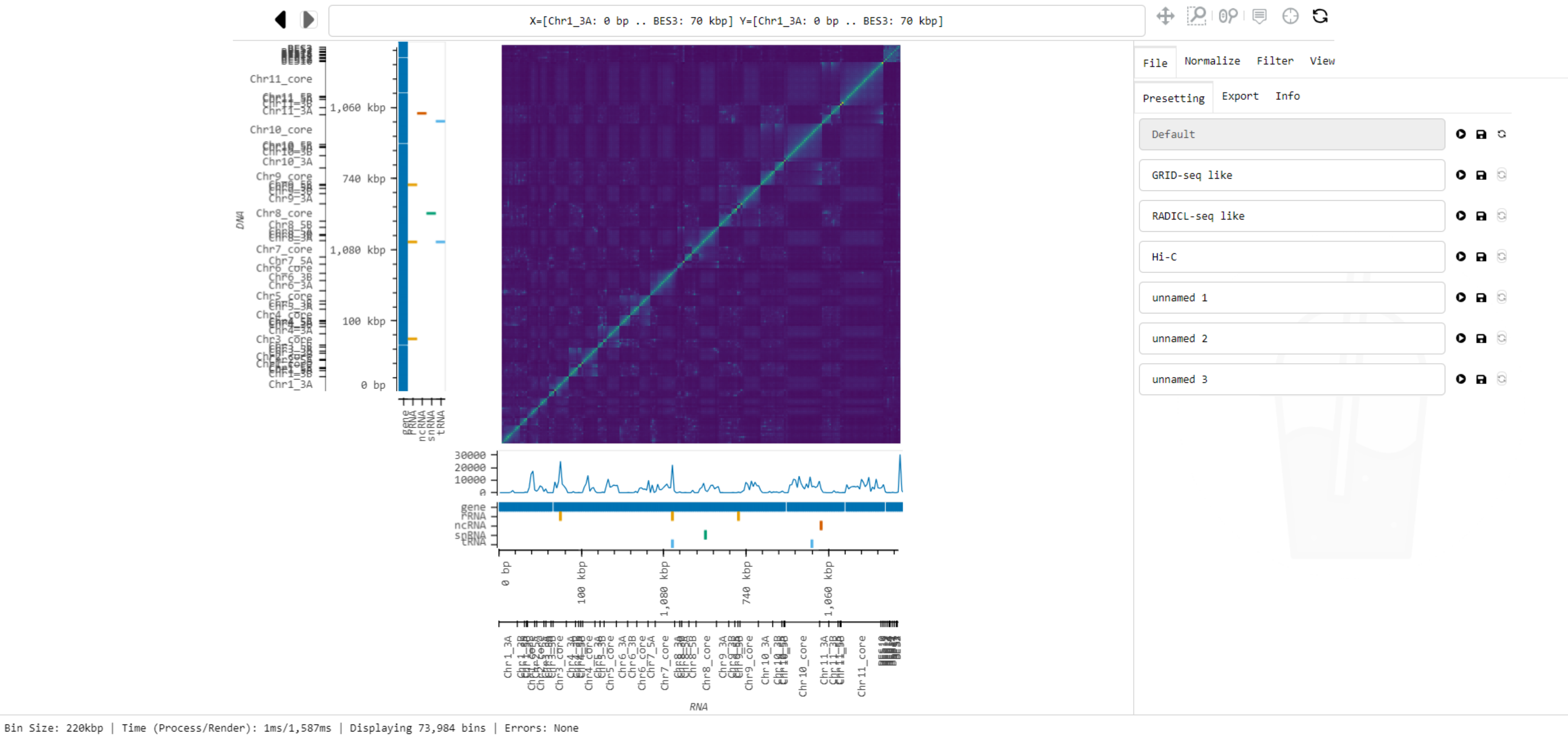
Here is a screenshot of Smoother in action:

Taking a tour 🚌

In this example, we install Smoother, download one of the sample datasets and run basic analyses. To do that we should have a terminal open:

We start by installing Smoother. Firstly, we create a new environment.

conda create -y -n smoother python=3.9
See the output of this command by clicking here.
    Collecting package metadata (current_repodata.json): done
    Solving environment: done==> WARNING: A newer version of conda exists. <==
current version: 4.10.3
latest version: 23.9.0

Please update conda by running

    $ conda update -n base conda


## Package Plan ##

environment location: /home/abarcons/miniconda3/envs/smoother

added / updated specs:
    - python=3.9


The following packages will be downloaded:

    package                    |            build
    ---------------------------|-----------------
    libnsl-2.0.0               |       hd590300_1          32 KB  conda-forge
    libsqlite-3.43.2           |       h2797004_0         820 KB  conda-forge
    tk-8.6.13                  |       h2797004_0         3.1 MB  conda-forge
    ------------------------------------------------------------
                                        Total:         4.0 MB

The following NEW packages will be INSTALLED:

_libgcc_mutex      conda-forge/linux-64::_libgcc_mutex-0.1-conda_forge
_openmp_mutex      conda-forge/linux-64::_openmp_mutex-4.5-2_gnu
bzip2              conda-forge/linux-64::bzip2-1.0.8-h7f98852_4
ca-certificates    conda-forge/linux-64::ca-certificates-2023.7.22-hbcca054_0
ld_impl_linux-64   conda-forge/linux-64::ld_impl_linux-64-2.40-h41732ed_0
libffi             conda-forge/linux-64::libffi-3.4.2-h7f98852_5
libgcc-ng          conda-forge/linux-64::libgcc-ng-13.2.0-h807b86a_2
libgomp            conda-forge/linux-64::libgomp-13.2.0-h807b86a_2
libnsl             conda-forge/linux-64::libnsl-2.0.0-hd590300_1
libsqlite          conda-forge/linux-64::libsqlite-3.43.2-h2797004_0
libuuid            conda-forge/linux-64::libuuid-2.38.1-h0b41bf4_0
libzlib            conda-forge/linux-64::libzlib-1.2.13-hd590300_5
ncurses            conda-forge/linux-64::ncurses-6.4-hcb278e6_0
openssl            conda-forge/linux-64::openssl-3.1.3-hd590300_0
pip                conda-forge/noarch::pip-23.2.1-pyhd8ed1ab_0
python             conda-forge/linux-64::python-3.9.18-h0755675_0_cpython
readline           conda-forge/linux-64::readline-8.2-h8228510_1
setuptools         conda-forge/noarch::setuptools-68.2.2-pyhd8ed1ab_0
tk                 conda-forge/linux-64::tk-8.6.13-h2797004_0
tzdata             conda-forge/noarch::tzdata-2023c-h71feb2d_0
wheel              conda-forge/noarch::wheel-0.41.2-pyhd8ed1ab_0
xz                 conda-forge/linux-64::xz-5.2.6-h166bdaf_0



Downloading and Extracting Packages
libsqlite-3.43.2     | 820 KB    | ######################################################## | 100%
libnsl-2.0.0         | 32 KB     | ######################################################## | 100%
tk-8.6.13            | 3.1 MB    | ######################################################## | 100%
Preparing transaction: done
Verifying transaction: done
Executing transaction: done
#
# To activate this environment, use
#
#     $ conda activate smoother
#
# To deactivate an active environment, use
#
#     $ conda deactivate

Secondly, we activate the environment.

conda activate smoother

Then, we install Smoother.

pip install biosmoother
See the output of this command by clicking here.
    (smoother) [ID@master name]$ pip install biosmoother
    Collecting biosmoother
    Obtaining dependency information for biosmoother from https://files.pythonhosted.org/packages/bd/a4/641ba3c9ab5704b8c7f52484d57cd7a83a363202aa7f0e383f7e06d31a73/biosmoother-1.0.1-py3-none-any.whl.metadata
    Downloading biosmoother-1.0.1-py3-none-any.whl.metadata (1.2 kB)
    Collecting libbiosmoother (from biosmoother)
    Obtaining dependency information for libbiosmoother from https://files.pythonhosted.org/packages/12/2e/2f40405174cb7a567a95f07e0dbcf7dfcc0d30aa614f60e0e33302cd8f1f/libbiosmoother-1.0.2-cp39-cp39-manylinux_2_17_x86_64.manylinux2014_x86_64.whl.metadata
    Downloading libbiosmoother-1.0.2-cp39-cp39-manylinux_2_17_x86_64.manylinux2014_x86_64.whl.metadata (1.2 kB)
    Collecting bokeh==2.3.2 (from biosmoother)
    Using cached bokeh-2.3.2-py3-none-any.whl
    Collecting psutil (from biosmoother)
    Using cached psutil-5.9.5-cp36-abi3-manylinux_2_12_x86_64.manylinux2010_x86_64.manylinux_2_17_x86_64.manylinux2014_x86_64.whl (282 kB)
    Collecting pybase64 (from biosmoother)
    Obtaining dependency information for pybase64 from https://files.pythonhosted.org/packages/c0/9c/47876c6af2bbcc5d7d376f6fb04e46536d8fabe22d5633888d303d50ce20/pybase64-1.3.1-cp39-cp39-manylinux_2_5_x86_64.manylinux1_x86_64.manylinux_2_17_x86_64.manylinux2014_x86_64.whl.metadata
    Downloading pybase64-1.3.1-cp39-cp39-manylinux_2_5_x86_64.manylinux1_x86_64.manylinux_2_17_x86_64.manylinux2014_x86_64.whl.metadata (7.9 kB)
    Collecting PyYAML>=3.10 (from bokeh==2.3.2->biosmoother)
    Obtaining dependency information for PyYAML>=3.10 from https://files.pythonhosted.org/packages/7d/39/472f2554a0f1e825bd7c5afc11c817cd7a2f3657460f7159f691fbb37c51/PyYAML-6.0.1-cp39-cp39-manylinux_2_17_x86_64.manylinux2014_x86_64.whl.metadata
    Using cached PyYAML-6.0.1-cp39-cp39-manylinux_2_17_x86_64.manylinux2014_x86_64.whl.metadata (2.1 kB)
    Collecting python-dateutil>=2.1 (from bokeh==2.3.2->biosmoother)
    Using cached python_dateutil-2.8.2-py2.py3-none-any.whl (247 kB)
    Collecting Jinja2>=2.9 (from bokeh==2.3.2->biosmoother)
    Using cached Jinja2-3.1.2-py3-none-any.whl (133 kB)
    Collecting numpy>=1.11.3 (from bokeh==2.3.2->biosmoother)
    Obtaining dependency information for numpy>=1.11.3 from https://files.pythonhosted.org/packages/75/cd/7ae0f2cd3fc68aea6cfb2b7e523842e1fa953adb38efabc110d27ba6e423/numpy-1.26.0-cp39-cp39-manylinux_2_17_x86_64.manylinux2014_x86_64.whl.metadata
    Using cached numpy-1.26.0-cp39-cp39-manylinux_2_17_x86_64.manylinux2014_x86_64.whl.metadata (58 kB)
    Collecting pillow>=7.1.0 (from bokeh==2.3.2->biosmoother)
    Obtaining dependency information for pillow>=7.1.0 from https://files.pythonhosted.org/packages/5d/cc/3345b8cf6f2b8c5ee33d59e3e2ddb693c45c4f3c88e10859f8b8abf9dc82/Pillow-10.0.1-cp39-cp39-manylinux_2_17_x86_64.manylinux2014_x86_64.whl.metadata
    Using cached Pillow-10.0.1-cp39-cp39-manylinux_2_17_x86_64.manylinux2014_x86_64.whl.metadata (9.5 kB)
    Collecting packaging>=16.8 (from bokeh==2.3.2->biosmoother)
    Obtaining dependency information for packaging>=16.8 from https://files.pythonhosted.org/packages/ec/1a/610693ac4ee14fcdf2d9bf3c493370e4f2ef7ae2e19217d7a237ff42367d/packaging-23.2-py3-none-any.whl.metadata
    Downloading packaging-23.2-py3-none-any.whl.metadata (3.2 kB)
    Collecting tornado>=5.1 (from bokeh==2.3.2->biosmoother)
    Obtaining dependency information for tornado>=5.1 from https://files.pythonhosted.org/packages/66/a5/e6da56c03ff61200d5a43cfb75ab09316fc0836aa7ee26b4e9dcbfc3ae85/tornado-6.3.3-cp38-abi3-manylinux_2_5_x86_64.manylinux1_x86_64.manylinux_2_17_x86_64.manylinux2014_x86_64.whl.metadata
    Using cached tornado-6.3.3-cp38-abi3-manylinux_2_5_x86_64.manylinux1_x86_64.manylinux_2_17_x86_64.manylinux2014_x86_64.whl.metadata (2.5 kB)
    Collecting typing-extensions>=3.7.4 (from bokeh==2.3.2->biosmoother)
    Obtaining dependency information for typing-extensions>=3.7.4 from https://files.pythonhosted.org/packages/24/21/7d397a4b7934ff4028987914ac1044d3b7d52712f30e2ac7a2ae5bc86dd0/typing_extensions-4.8.0-py3-none-any.whl.metadata
    Using cached typing_extensions-4.8.0-py3-none-any.whl.metadata (3.0 kB)
    Collecting scipy (from libbiosmoother->biosmoother)
    Obtaining dependency information for scipy from https://files.pythonhosted.org/packages/88/8c/9d1f74196c296046af1f20e6d3fc7fbb27387282315e1643f450bba14329/scipy-1.11.3-cp39-cp39-manylinux_2_17_x86_64.manylinux2014_x86_64.whl.metadata
    Downloading scipy-1.11.3-cp39-cp39-manylinux_2_17_x86_64.manylinux2014_x86_64.whl.metadata (60 kB)
        ━━━━━━━━━━━━━━━━━━━━━━━━━━━━━━━━━━━━━━━━ 60.4/60.4 kB 1.3 MB/s eta 0:00:00
    Collecting statsmodels (from libbiosmoother->biosmoother)
    Using cached statsmodels-0.14.0-cp39-cp39-manylinux_2_17_x86_64.manylinux2014_x86_64.whl (10.1 MB)
    Collecting scikit-learn (from libbiosmoother->biosmoother)
    Obtaining dependency information for scikit-learn from https://files.pythonhosted.org/packages/af/ad/329a88013936e4372181c0e275c19aa6130b0835876726944b811af5a856/scikit_learn-1.3.1-cp39-cp39-manylinux_2_17_x86_64.manylinux2014_x86_64.whl.metadata
    Using cached scikit_learn-1.3.1-cp39-cp39-manylinux_2_17_x86_64.manylinux2014_x86_64.whl.metadata (11 kB)
    Collecting drawSvg==1.9.0 (from libbiosmoother->biosmoother)
    Using cached drawSvg-1.9.0-py3-none-any.whl (26 kB)
    Collecting cairoSVG (from drawSvg==1.9.0->libbiosmoother->biosmoother)
    Obtaining dependency information for cairoSVG from https://files.pythonhosted.org/packages/01/a5/1866b42151f50453f1a0d28fc4c39f5be5f412a2e914f33449c42daafdf1/CairoSVG-2.7.1-py3-none-any.whl.metadata
    Using cached CairoSVG-2.7.1-py3-none-any.whl.metadata (2.7 kB)
    Collecting imageio (from drawSvg==1.9.0->libbiosmoother->biosmoother)
    Obtaining dependency information for imageio from https://files.pythonhosted.org/packages/f6/37/e21e6f38b93878ba80302e95b8ccd4718d80f0c53055ccae343e606b1e2d/imageio-2.31.5-py3-none-any.whl.metadata
    Downloading imageio-2.31.5-py3-none-any.whl.metadata (4.6 kB)
    Collecting MarkupSafe>=2.0 (from Jinja2>=2.9->bokeh==2.3.2->biosmoother)
    Obtaining dependency information for MarkupSafe>=2.0 from https://files.pythonhosted.org/packages/de/63/cb7e71984e9159ec5f45b5e81e896c8bdd0e45fe3fc6ce02ab497f0d790e/MarkupSafe-2.1.3-cp39-cp39-manylinux_2_17_x86_64.manylinux2014_x86_64.whl.metadata
    Using cached MarkupSafe-2.1.3-cp39-cp39-manylinux_2_17_x86_64.manylinux2014_x86_64.whl.metadata (3.0 kB)
    Collecting six>=1.5 (from python-dateutil>=2.1->bokeh==2.3.2->biosmoother)
    Using cached six-1.16.0-py2.py3-none-any.whl (11 kB)
    Collecting joblib>=1.1.1 (from scikit-learn->libbiosmoother->biosmoother)
    Obtaining dependency information for joblib>=1.1.1 from https://files.pythonhosted.org/packages/10/40/d551139c85db202f1f384ba8bcf96aca2f329440a844f924c8a0040b6d02/joblib-1.3.2-py3-none-any.whl.metadata
    Using cached joblib-1.3.2-py3-none-any.whl.metadata (5.4 kB)
    Collecting threadpoolctl>=2.0.0 (from scikit-learn->libbiosmoother->biosmoother)
    Obtaining dependency information for threadpoolctl>=2.0.0 from https://files.pythonhosted.org/packages/81/12/fd4dea011af9d69e1cad05c75f3f7202cdcbeac9b712eea58ca779a72865/threadpoolctl-3.2.0-py3-none-any.whl.metadata
    Using cached threadpoolctl-3.2.0-py3-none-any.whl.metadata (10.0 kB)
    Collecting pandas>=1.0 (from statsmodels->libbiosmoother->biosmoother)
    Obtaining dependency information for pandas>=1.0 from https://files.pythonhosted.org/packages/bc/7e/a9e11bd272e3135108892b6230a115568f477864276181eada3a35d03237/pandas-2.1.1-cp39-cp39-manylinux_2_17_x86_64.manylinux2014_x86_64.whl.metadata
    Using cached pandas-2.1.1-cp39-cp39-manylinux_2_17_x86_64.manylinux2014_x86_64.whl.metadata (18 kB)
    Collecting patsy>=0.5.2 (from statsmodels->libbiosmoother->biosmoother)
    Using cached patsy-0.5.3-py2.py3-none-any.whl (233 kB)
    Collecting pytz>=2020.1 (from pandas>=1.0->statsmodels->libbiosmoother->biosmoother)
    Obtaining dependency information for pytz>=2020.1 from https://files.pythonhosted.org/packages/32/4d/aaf7eff5deb402fd9a24a1449a8119f00d74ae9c2efa79f8ef9994261fc2/pytz-2023.3.post1-py2.py3-none-any.whl.metadata
    Using cached pytz-2023.3.post1-py2.py3-none-any.whl.metadata (22 kB)
    Collecting tzdata>=2022.1 (from pandas>=1.0->statsmodels->libbiosmoother->biosmoother)
    Using cached tzdata-2023.3-py2.py3-none-any.whl (341 kB)
    Collecting cairocffi (from cairoSVG->drawSvg==1.9.0->libbiosmoother->biosmoother)
    Obtaining dependency information for cairocffi from https://files.pythonhosted.org/packages/17/be/a5d2c16317c6a890502725970589ae7f06cfc66b2e6916ba0a86973403c8/cairocffi-1.6.1-py3-none-any.whl.metadata
    Using cached cairocffi-1.6.1-py3-none-any.whl.metadata (3.3 kB)
    Collecting cssselect2 (from cairoSVG->drawSvg==1.9.0->libbiosmoother->biosmoother)
    Using cached cssselect2-0.7.0-py3-none-any.whl (15 kB)
    Collecting defusedxml (from cairoSVG->drawSvg==1.9.0->libbiosmoother->biosmoother)
    Using cached defusedxml-0.7.1-py2.py3-none-any.whl (25 kB)
    Collecting tinycss2 (from cairoSVG->drawSvg==1.9.0->libbiosmoother->biosmoother)
    Using cached tinycss2-1.2.1-py3-none-any.whl (21 kB)
    Collecting cffi>=1.1.0 (from cairocffi->cairoSVG->drawSvg==1.9.0->libbiosmoother->biosmoother)
    Obtaining dependency information for cffi>=1.1.0 from https://files.pythonhosted.org/packages/ea/ac/e9e77bc385729035143e54cc8c4785bd480eaca9df17565963556b0b7a93/cffi-1.16.0-cp39-cp39-manylinux_2_17_x86_64.manylinux2014_x86_64.whl.metadata
    Downloading cffi-1.16.0-cp39-cp39-manylinux_2_17_x86_64.manylinux2014_x86_64.whl.metadata (1.5 kB)
    Collecting webencodings (from cssselect2->cairoSVG->drawSvg==1.9.0->libbiosmoother->biosmoother)
    Using cached webencodings-0.5.1-py2.py3-none-any.whl (11 kB)
    Collecting pycparser (from cffi>=1.1.0->cairocffi->cairoSVG->drawSvg==1.9.0->libbiosmoother->biosmoother)
    Using cached pycparser-2.21-py2.py3-none-any.whl (118 kB)
    Downloading biosmoother-1.0.1-py3-none-any.whl (339 kB)
    ━━━━━━━━━━━━━━━━━━━━━━━━━━━━━━━━━━━━━━━━ 339.4/339.4 kB 6.9 MB/s eta 0:00:00
    Downloading libbiosmoother-1.0.2-cp39-cp39-manylinux_2_17_x86_64.manylinux2014_x86_64.whl (1.6 MB)
    ━━━━━━━━━━━━━━━━━━━━━━━━━━━━━━━━━━━━━━━━ 1.6/1.6 MB 4.4 MB/s eta 0:00:00
    Downloading pybase64-1.3.1-cp39-cp39-manylinux_2_5_x86_64.manylinux1_x86_64.manylinux_2_17_x86_64.manylinux2014_x86_64.whl (64 kB)
    ━━━━━━━━━━━━━━━━━━━━━━━━━━━━━━━━━━━━━━━━ 64.9/64.9 kB 11.4 MB/s eta 0:00:00
    Using cached numpy-1.26.0-cp39-cp39-manylinux_2_17_x86_64.manylinux2014_x86_64.whl (18.2 MB)
    Downloading packaging-23.2-py3-none-any.whl (53 kB)
    ━━━━━━━━━━━━━━━━━━━━━━━━━━━━━━━━━━━━━━━━ 53.0/53.0 kB 10.4 MB/s eta 0:00:00
    Using cached Pillow-10.0.1-cp39-cp39-manylinux_2_17_x86_64.manylinux2014_x86_64.whl (3.5 MB)
    Using cached PyYAML-6.0.1-cp39-cp39-manylinux_2_17_x86_64.manylinux2014_x86_64.whl (738 kB)
    Using cached tornado-6.3.3-cp38-abi3-manylinux_2_5_x86_64.manylinux1_x86_64.manylinux_2_17_x86_64.manylinux2014_x86_64.whl (427 kB)
    Using cached typing_extensions-4.8.0-py3-none-any.whl (31 kB)
    Using cached scikit_learn-1.3.1-cp39-cp39-manylinux_2_17_x86_64.manylinux2014_x86_64.whl (10.9 MB)
    Downloading scipy-1.11.3-cp39-cp39-manylinux_2_17_x86_64.manylinux2014_x86_64.whl (36.6 MB)
    ━━━━━━━━━━━━━━━━━━━━━━━━━━━━━━━━━━━━━━━━ 36.6/36.6 MB 10.8 MB/s eta 0:00:00
    Using cached joblib-1.3.2-py3-none-any.whl (302 kB)
    Using cached MarkupSafe-2.1.3-cp39-cp39-manylinux_2_17_x86_64.manylinux2014_x86_64.whl (25 kB)
    Using cached pandas-2.1.1-cp39-cp39-manylinux_2_17_x86_64.manylinux2014_x86_64.whl (12.3 MB)
    Using cached threadpoolctl-3.2.0-py3-none-any.whl (15 kB)
    Using cached CairoSVG-2.7.1-py3-none-any.whl (43 kB)
    Downloading imageio-2.31.5-py3-none-any.whl (313 kB)
    ━━━━━━━━━━━━━━━━━━━━━━━━━━━━━━━━━━━━━━━━ 313.2/313.2 kB 10.8 MB/s eta 0:00:00
    Using cached pytz-2023.3.post1-py2.py3-none-any.whl (502 kB)
    Using cached cairocffi-1.6.1-py3-none-any.whl (75 kB)
    Downloading cffi-1.16.0-cp39-cp39-manylinux_2_17_x86_64.manylinux2014_x86_64.whl (443 kB)
    ━━━━━━━━━━━━━━━━━━━━━━━━━━━━━━━━━━━━━━━━ 443.4/443.4 kB 39.7 MB/s eta 0:00:00
    Installing collected packages: webencodings, pytz, tzdata, typing-extensions, tornado, tinycss2, threadpoolctl, six, PyYAML, pycparser, pybase64, psutil, pillow, packaging, numpy, MarkupSafe, joblib, defusedxml, scipy, python-dateutil, patsy, Jinja2, imageio, cssselect2, cffi, scikit-learn, pandas, cairocffi, bokeh, statsmodels, cairoSVG, drawSvg, libbiosmoother, biosmoother
    Successfully installed Jinja2-3.1.2 MarkupSafe-2.1.3 PyYAML-6.0.1 biosmoother-1.0.1 bokeh-2.3.2 cairoSVG-2.7.1 cairocffi-1.6.1 cffi-1.16.0 cssselect2-0.7.0 defusedxml-0.7.1 drawSvg-1.9.0 imageio-2.31.5 joblib-1.3.2 libbiosmoother-1.0.2 numpy-1.26.0 packaging-23.2 pandas-2.1.1 patsy-0.5.3 pillow-10.0.1 psutil-5.9.5 pybase64-1.3.1 pycparser-2.21 python-dateutil-2.8.2 pytz-2023.3.post1 scikit-learn-1.3.1 scipy-1.11.3 six-1.16.0 statsmodels-0.14.0 threadpoolctl-3.2.0 tinycss2-1.2.1 tornado-6.3.3 typing-extensions-4.8.0 tzdata-2023.3 webencodings-0.5.1

Finally, we install further requirements for Smoother.

conda install -y nodejs cairo
See the output of this command by clicking here.Collecting package metadata (current_repodata.json): done
Solving environment: done


==> WARNING: A newer version of conda exists. <==
current version: 4.10.3
latest version: 23.9.0

Please update conda by running

    $ conda update -n base conda



## Package Plan ##

environment location: /home/abarcons/miniconda3/envs/smoother

added / updated specs:
    - cairo
    - nodejs


The following packages will be downloaded:

    package                    |            build
    ---------------------------|-----------------
    cairo-1.16.0               |    h0c91306_1017         1.1 MB  conda-forge
    libxcb-1.15                |       h0b41bf4_0         375 KB  conda-forge
    nodejs-20.8.0              |       hb753e55_0        16.3 MB  conda-forge
    pixman-0.42.2              |       h59595ed_0         376 KB  conda-forge
    xorg-libx11-1.8.6          |       h8ee46fc_0         809 KB  conda-forge
    xorg-libxrender-0.9.11     |       hd590300_0          37 KB  conda-forge
    ------------------------------------------------------------
                                        Total:        18.9 MB

The following NEW packages will be INSTALLED:

cairo              conda-forge/linux-64::cairo-1.16.0-h0c91306_1017
expat              conda-forge/linux-64::expat-2.5.0-hcb278e6_1
font-ttf-dejavu-s~ conda-forge/noarch::font-ttf-dejavu-sans-mono-2.37-hab24e00_0
font-ttf-inconsol~ conda-forge/noarch::font-ttf-inconsolata-3.000-h77eed37_0
font-ttf-source-c~ conda-forge/noarch::font-ttf-source-code-pro-2.038-h77eed37_0
font-ttf-ubuntu    conda-forge/noarch::font-ttf-ubuntu-0.83-hab24e00_0
fontconfig         conda-forge/linux-64::fontconfig-2.14.2-h14ed4e7_0
fonts-conda-ecosy~ conda-forge/noarch::fonts-conda-ecosystem-1-0
fonts-conda-forge  conda-forge/noarch::fonts-conda-forge-1-0
freetype           conda-forge/linux-64::freetype-2.12.1-h267a509_2
gettext            conda-forge/linux-64::gettext-0.21.1-h27087fc_0
icu                conda-forge/linux-64::icu-73.2-h59595ed_0
libexpat           conda-forge/linux-64::libexpat-2.5.0-hcb278e6_1
libglib            conda-forge/linux-64::libglib-2.78.0-hebfc3b9_0
libiconv           conda-forge/linux-64::libiconv-1.17-h166bdaf_0
libpng             conda-forge/linux-64::libpng-1.6.39-h753d276_0
libstdcxx-ng       conda-forge/linux-64::libstdcxx-ng-13.2.0-h7e041cc_2
libuv              conda-forge/linux-64::libuv-1.46.0-hd590300_0
libxcb             conda-forge/linux-64::libxcb-1.15-h0b41bf4_0
nodejs             conda-forge/linux-64::nodejs-20.8.0-hb753e55_0
pcre2              conda-forge/linux-64::pcre2-10.40-hc3806b6_0
pixman             conda-forge/linux-64::pixman-0.42.2-h59595ed_0
pthread-stubs      conda-forge/linux-64::pthread-stubs-0.4-h36c2ea0_1001
xorg-kbproto       conda-forge/linux-64::xorg-kbproto-1.0.7-h7f98852_1002
xorg-libice        conda-forge/linux-64::xorg-libice-1.1.1-hd590300_0
xorg-libsm         conda-forge/linux-64::xorg-libsm-1.2.4-h7391055_0
xorg-libx11        conda-forge/linux-64::xorg-libx11-1.8.6-h8ee46fc_0
xorg-libxau        conda-forge/linux-64::xorg-libxau-1.0.11-hd590300_0
xorg-libxdmcp      conda-forge/linux-64::xorg-libxdmcp-1.1.3-h7f98852_0
xorg-libxext       conda-forge/linux-64::xorg-libxext-1.3.4-h0b41bf4_2
xorg-libxrender    conda-forge/linux-64::xorg-libxrender-0.9.11-hd590300_0
xorg-renderproto   conda-forge/linux-64::xorg-renderproto-0.11.1-h7f98852_1002
xorg-xextproto     conda-forge/linux-64::xorg-xextproto-7.3.0-h0b41bf4_1003
xorg-xproto        conda-forge/linux-64::xorg-xproto-7.0.31-h7f98852_1007
zlib               conda-forge/linux-64::zlib-1.2.13-hd590300_5



Downloading and Extracting Packages
libxcb-1.15          | 375 KB    | ############################################ | 100%
cairo-1.16.0         | 1.1 MB    | ############################################ | 100%
nodejs-20.8.0        | 16.3 MB   | ############################################ | 100%
pixman-0.42.2        | 376 KB    | ############################################ | 100%
xorg-libx11-1.8.6    | 809 KB    | ############################################ | 100%
xorg-libxrender-0.9. | 37 KB     | ############################################ | 100%
Preparing transaction: done
Verifying transaction: done
Executing transaction: done

We download one example Smoother index.

wget https://syncandshare.lrz.de/dl/fiTWvK4pxwB2TQkMSrzzDJ/t_brucei_hi_c.smoother_index.zip
See the output of this command by clicking here.
    --2023-10-11 14:20:52--  https://syncandshare.lrz.de/dl/fiTWvK4pxwB2TQkMSrzzDJ/t_brucei_hi_c.smoother_index.zip
    Resolving syncandshare.lrz.de (syncandshare.lrz.de)... 129.187.255.213
    Connecting to syncandshare.lrz.de (syncandshare.lrz.de)|129.187.255.213|:443... connected.
    HTTP request sent, awaiting response... 200 OK
    Length: 1297169622 (1.2G) [application/x-zip-compressed]
    Saving to: 't_brucei_hi_c.smoother_index.zip'100%[===============================================================================================>] 1,297,169,622 58.2MB/s   in 20s

2023-10-11 14:21:13 (60.6 MB/s) - 't_brucei_hi_c.smoother_index.zip' saved [1297169622/1297169622]

We unzip the example Smoother index.

unzip t_brucei_hi_c.smoother_index.zip
See the output of this command by clicking here.
    Archive:  t_brucei_hi_c.smoother_index.zip
    creating: t_brucei_hi_c.smoother_index/
    extracting: t_brucei_hi_c.smoother_index/sps.corners
    inflating: t_brucei_hi_c.smoother_index/anno.desc
    inflating: t_brucei_hi_c.smoother_index/anno.intervals
    inflating: t_brucei_hi_c.smoother_index/session.json
    inflating: t_brucei_hi_c.smoother_index/default_session.json
    inflating: t_brucei_hi_c.smoother_index/sps.overlays
    inflating: t_brucei_hi_c.smoother_index/sps.coords
    inflating: t_brucei_hi_c.smoother_index/anno.datasets
    inflating: t_brucei_hi_c.smoother_index/sps.prefix_sums
    inflating: t_brucei_hi_c.smoother_index/sps.datasets

We load the index on Smoother.

biosmoother serve t_brucei_hi_c.smoother_index --show
See the output of this command by clicking here.
    loading index...
    done loading.
    starting biosmoother server at: http://localhost:5006/biosmoother
    WARNING: the version of libSps that was used to create this index is different from the current version. This may lead to undefined behavior.
    Version in index: 0.4.1-ca0d905-2023-09-05-14:22:50
    Current version: 1.0.0-5c093ba-2023-10-10-12:35:53
    WARNING: the version of libBioSmoother that was used to create this index is different from the current version. This may lead to undefined behavior.
    Version in index: 0.5.0-ce0be2e-2023-09-11-12:53:38
    Current version: 1.0.3-8512484-2023-10-11-17:36:56

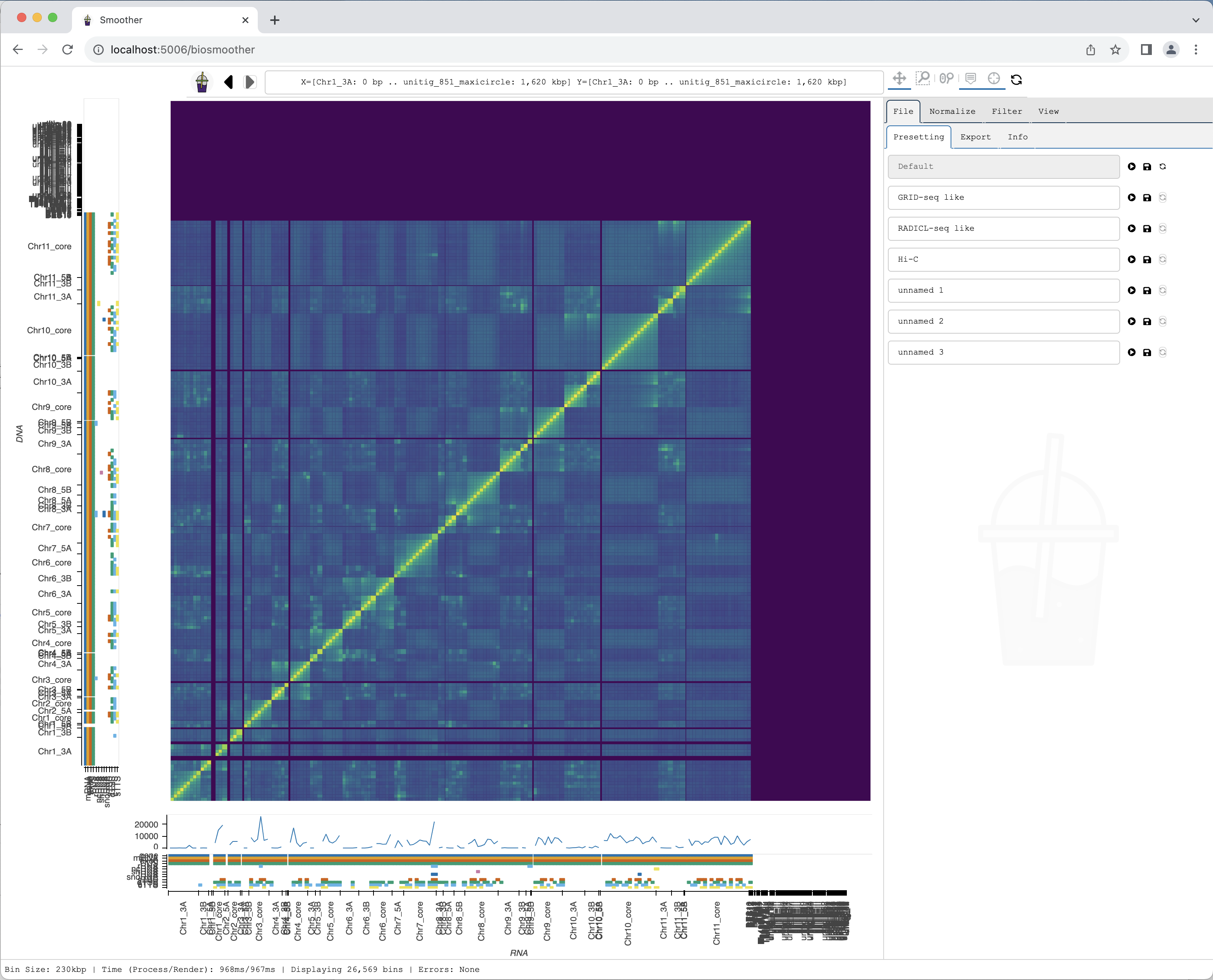
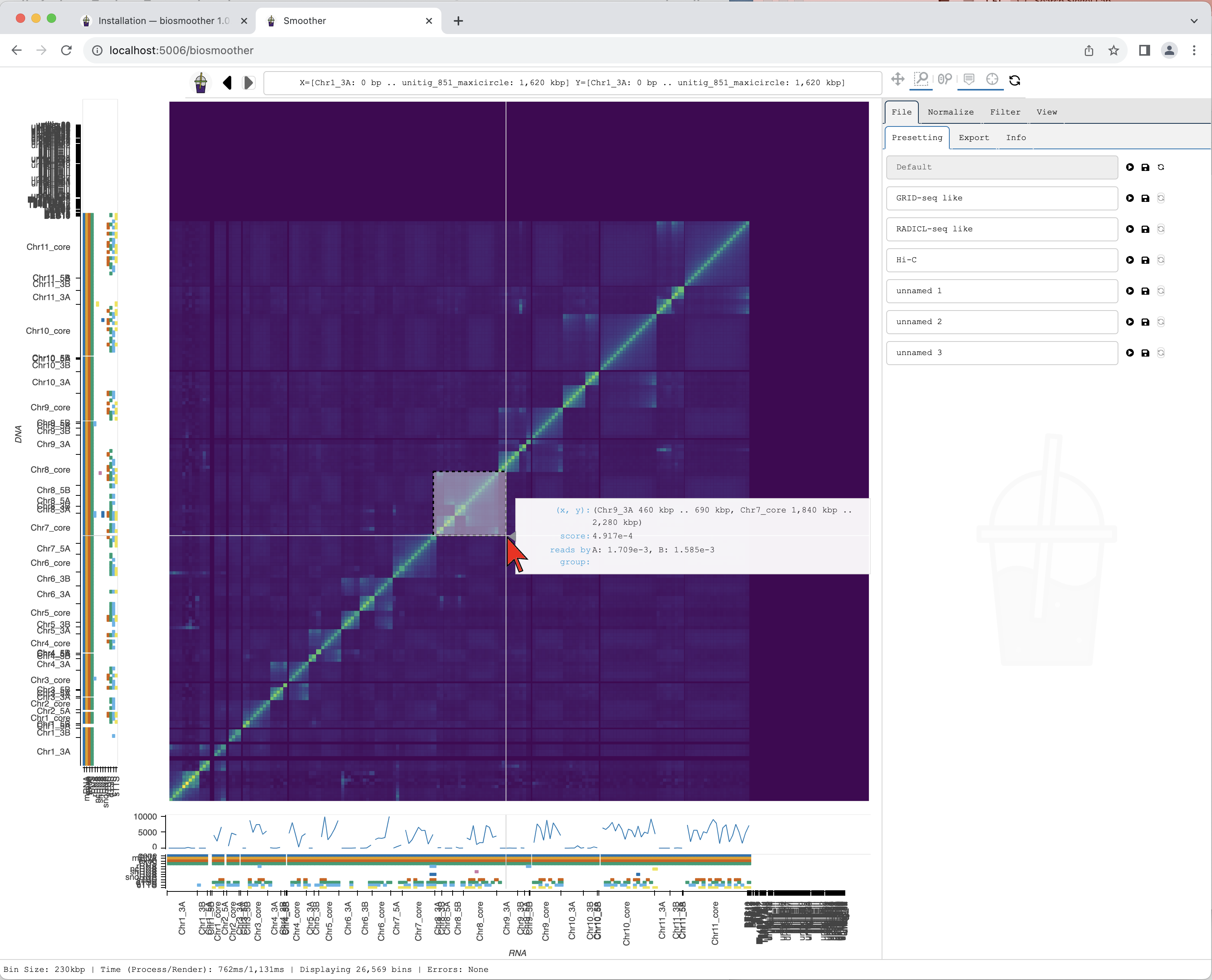
Since we used the --show option, a browser tab should open. In it we should see our heatmap after a few seconds:

Changing mapping quality filter

We will now perform some example analysis and navigation on Smoother.

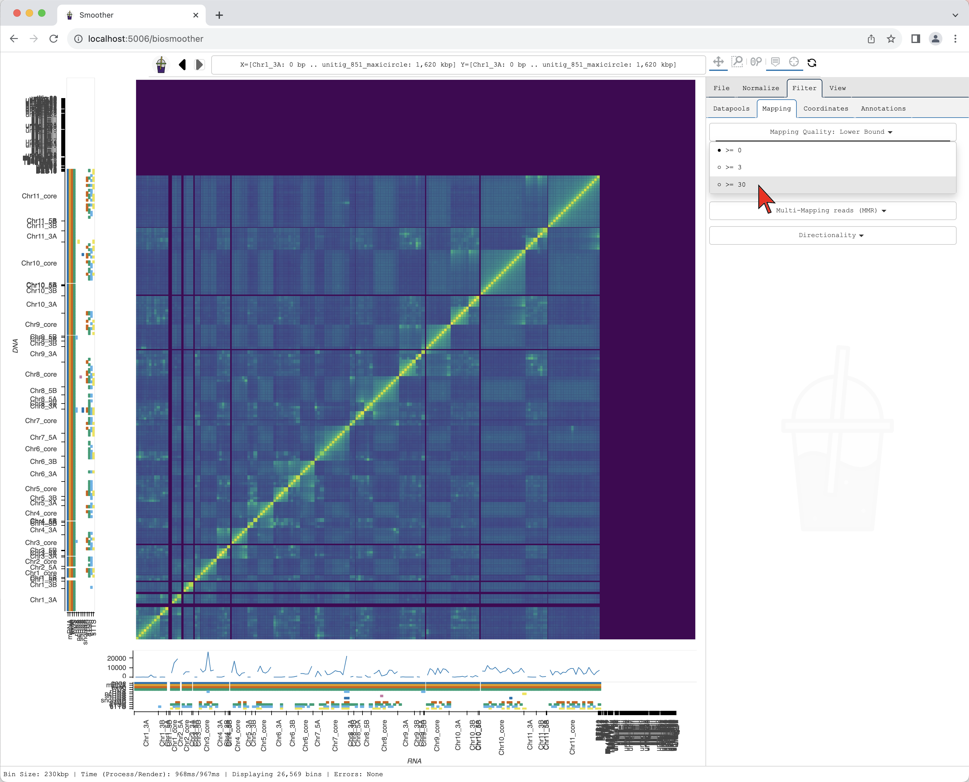
We start by changing the mapping quality filter. First, we select the Filter tab.

We then select the Filter->Mapping subtab.

In the dropdown menu Mapping Quality: Lower Bound we can select the threshold for mapping quality.

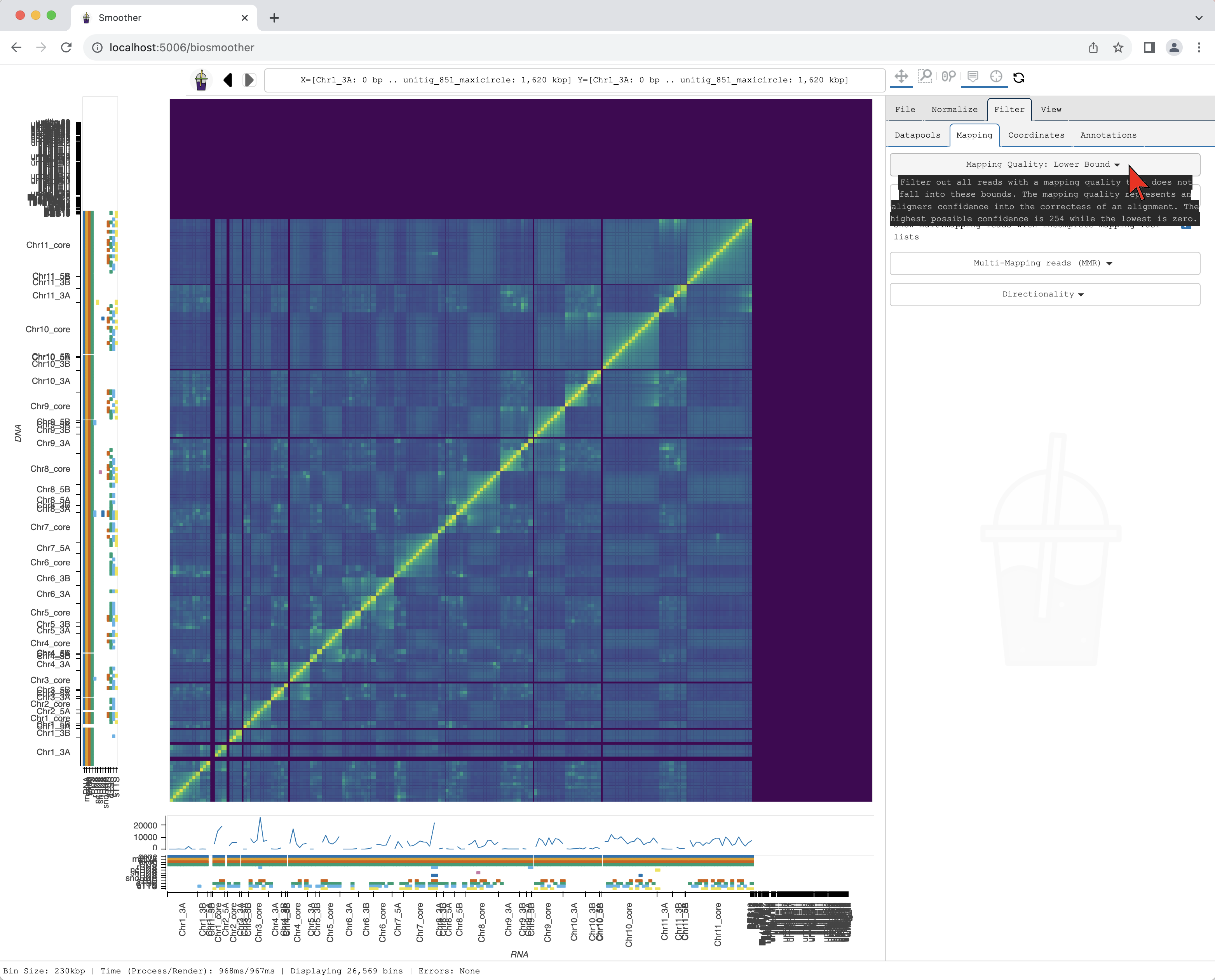
Here, we select >=30 that will filter out the reads with mapping quality score below 30.

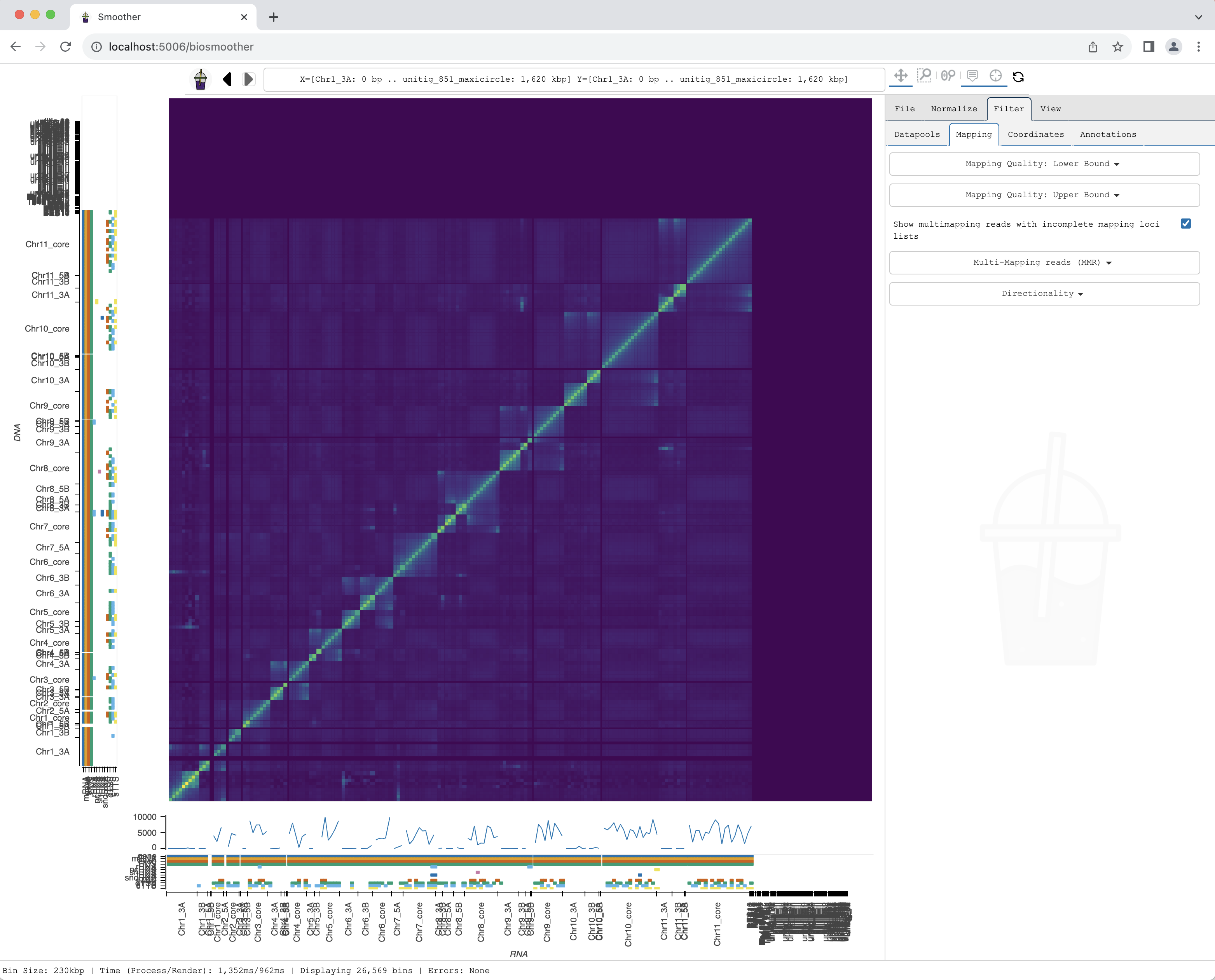
After selecting the filter, the heatmap re-renders with the updated mapping quality filter.

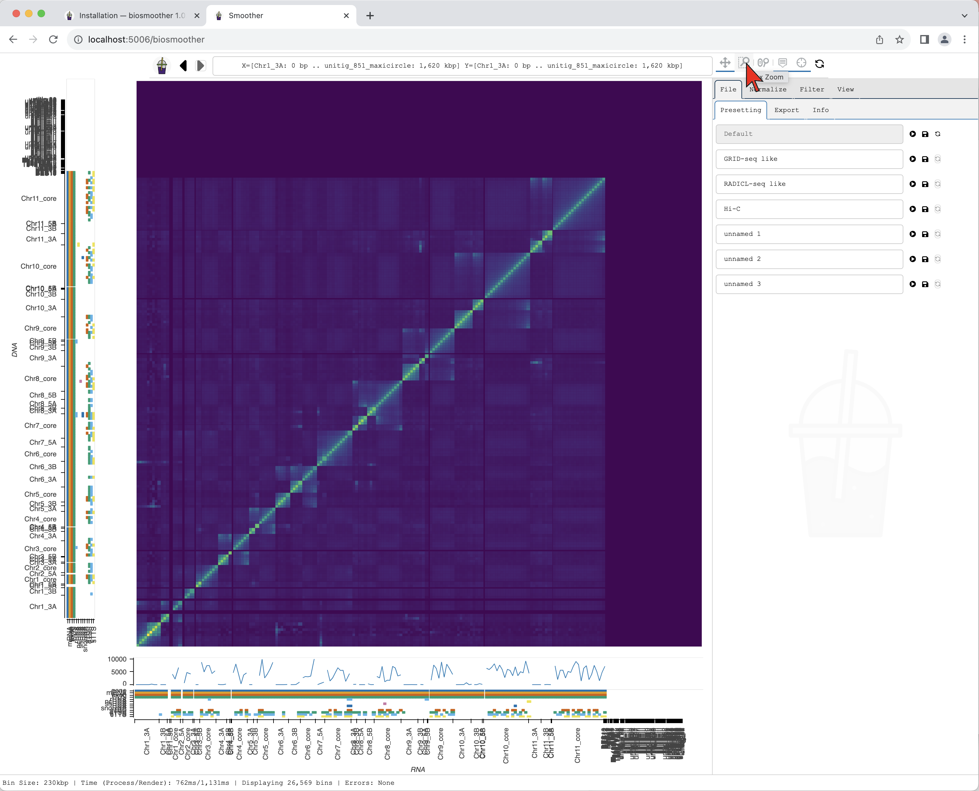
Zooming into a region of interest

We now can zoom to a particular genomic location of interest, for example using the Box zoom.

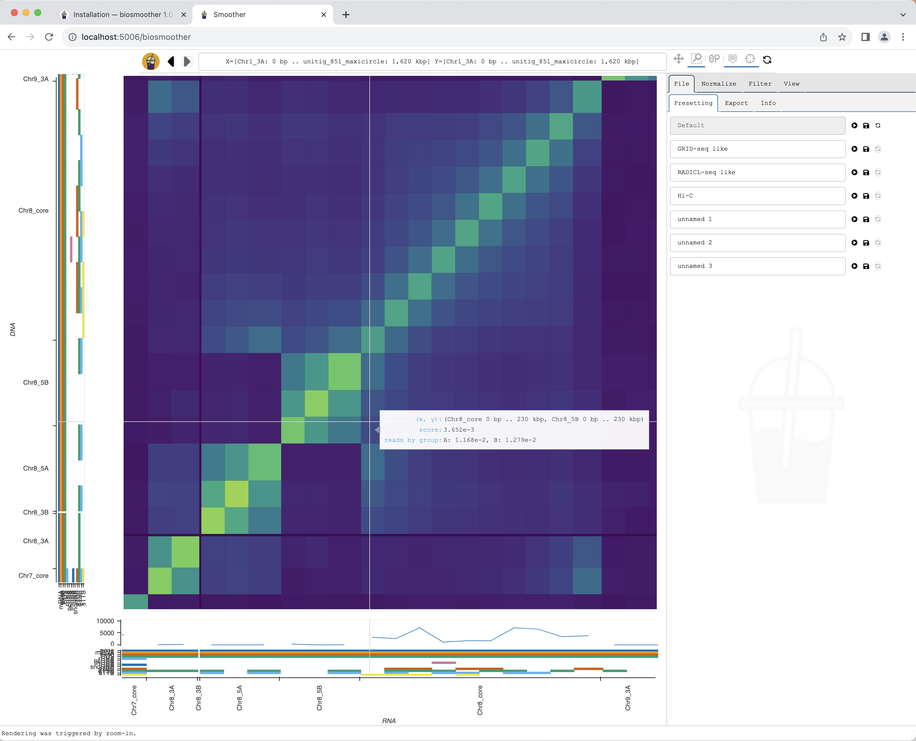
We draw a box around the region of interest.

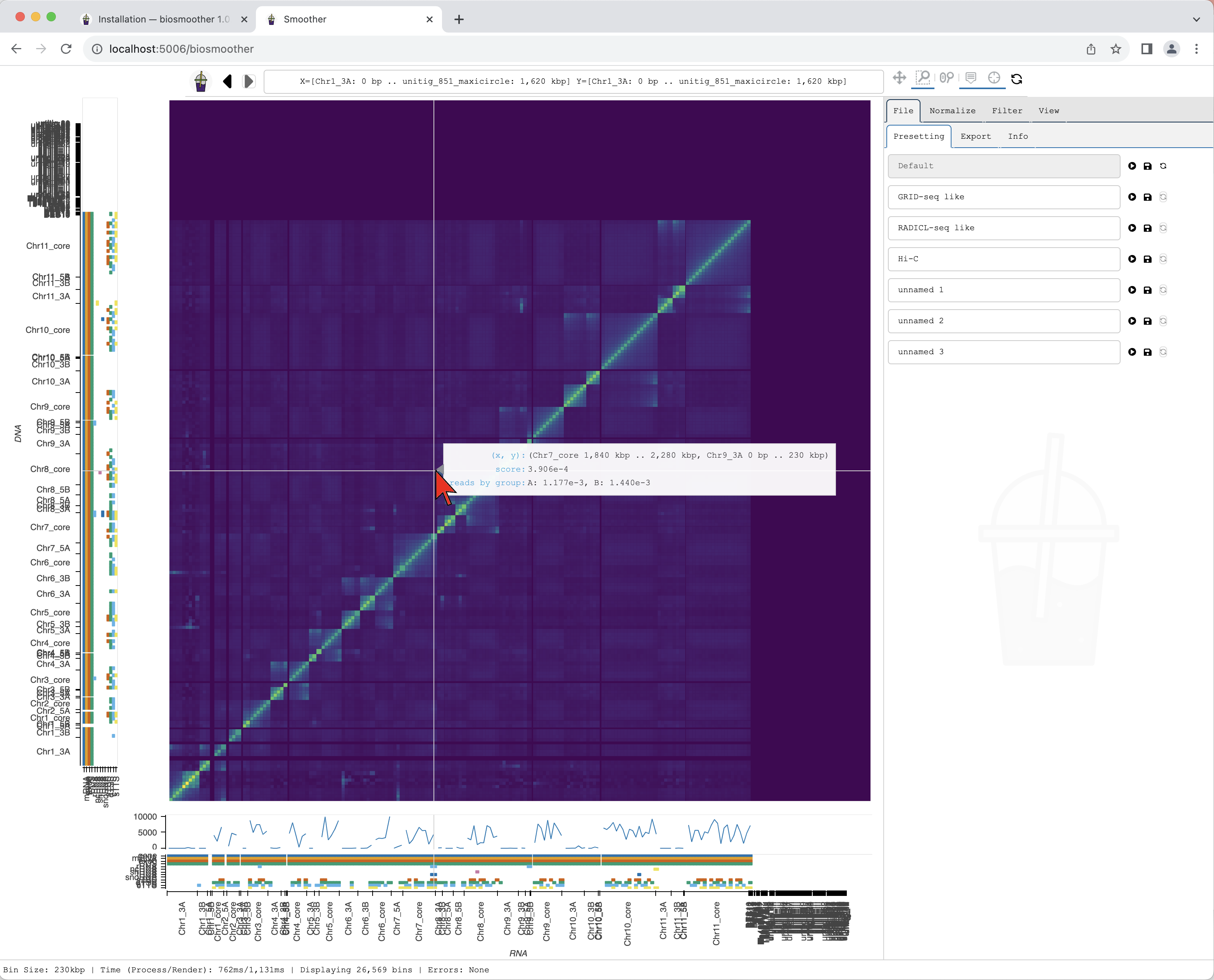
Smoother renders the zoomed region. While Smoother is rendering there is a yellow background on the top left icon.

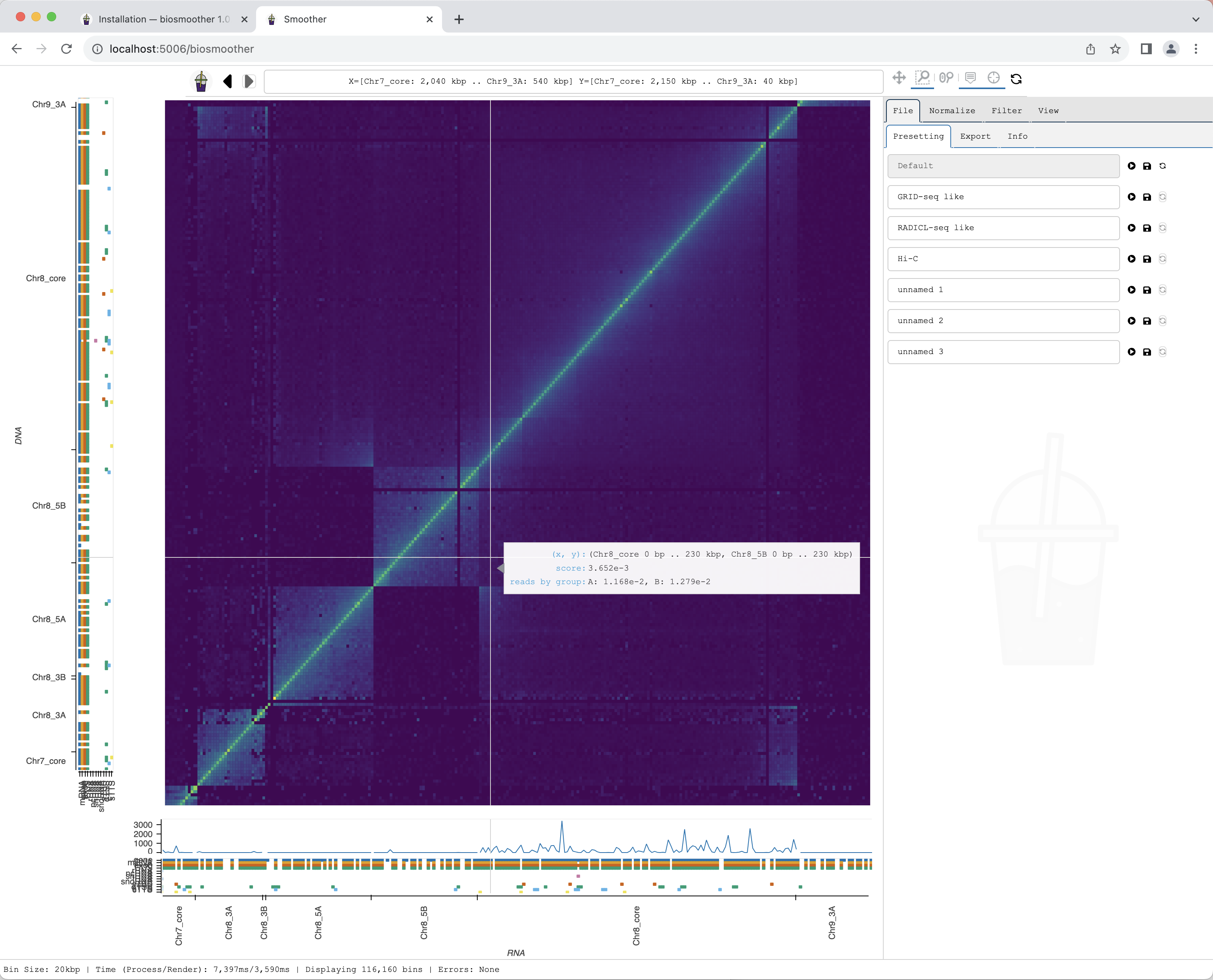
The new region is rendered.

Exporting a picture

We can now export a picture of the zoomed in region of interest. To do so we have to select the File->Export subtab.

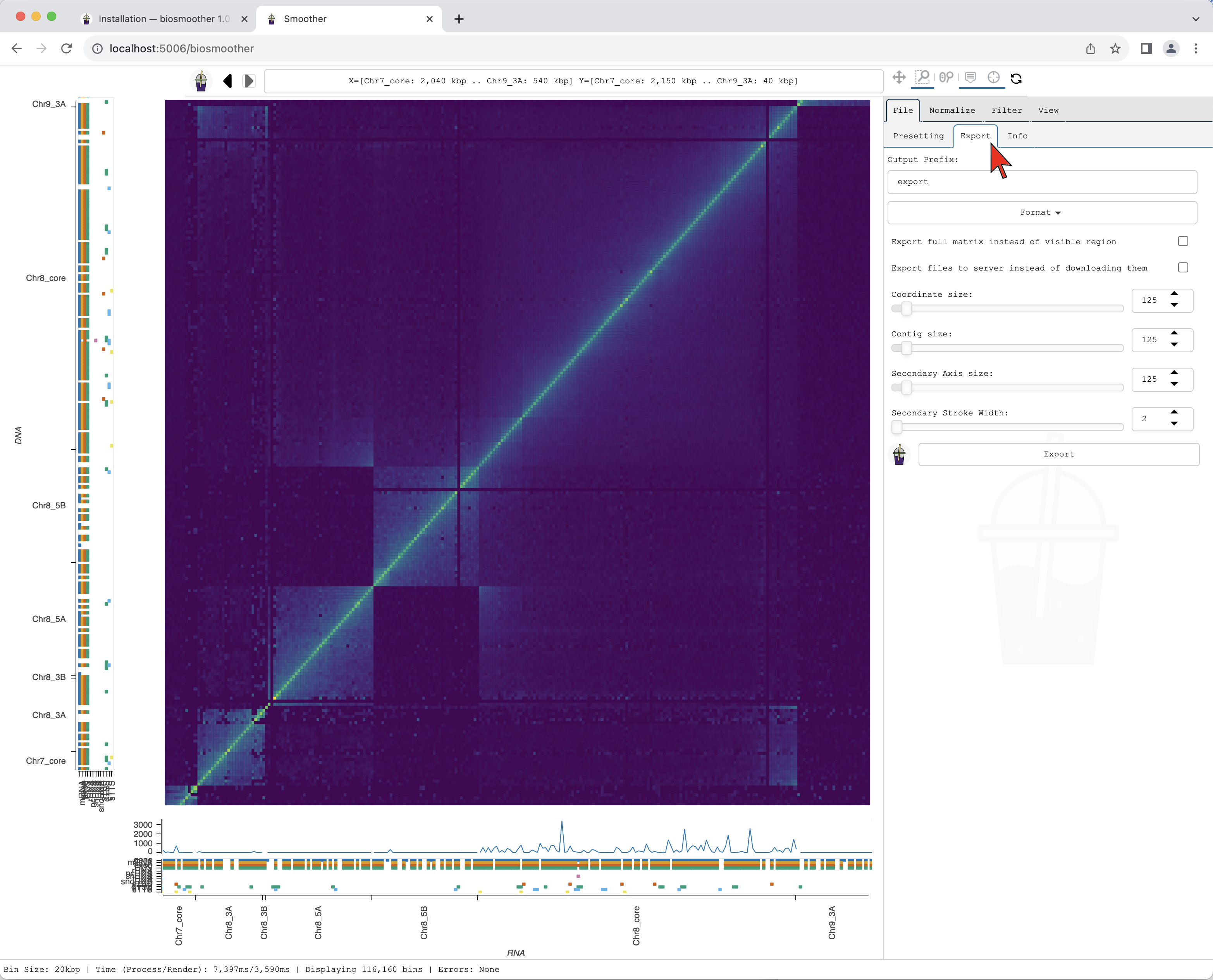
We then select the format we want in the dropdown menu Format.

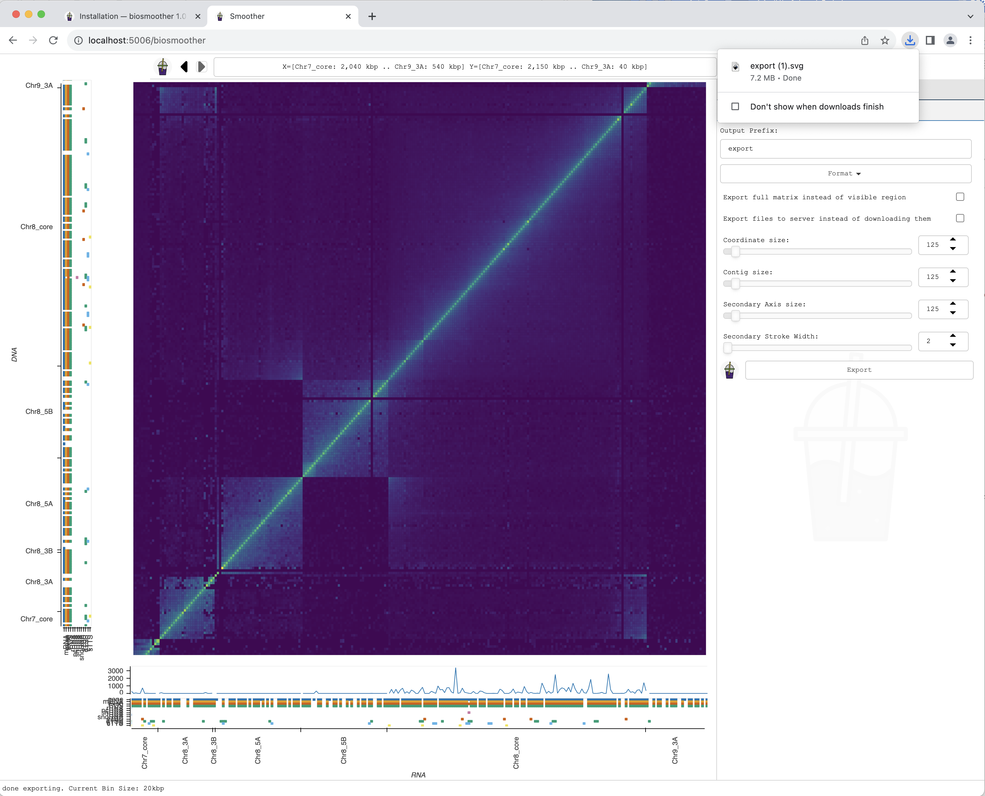
We can then press the Export button to save the file.

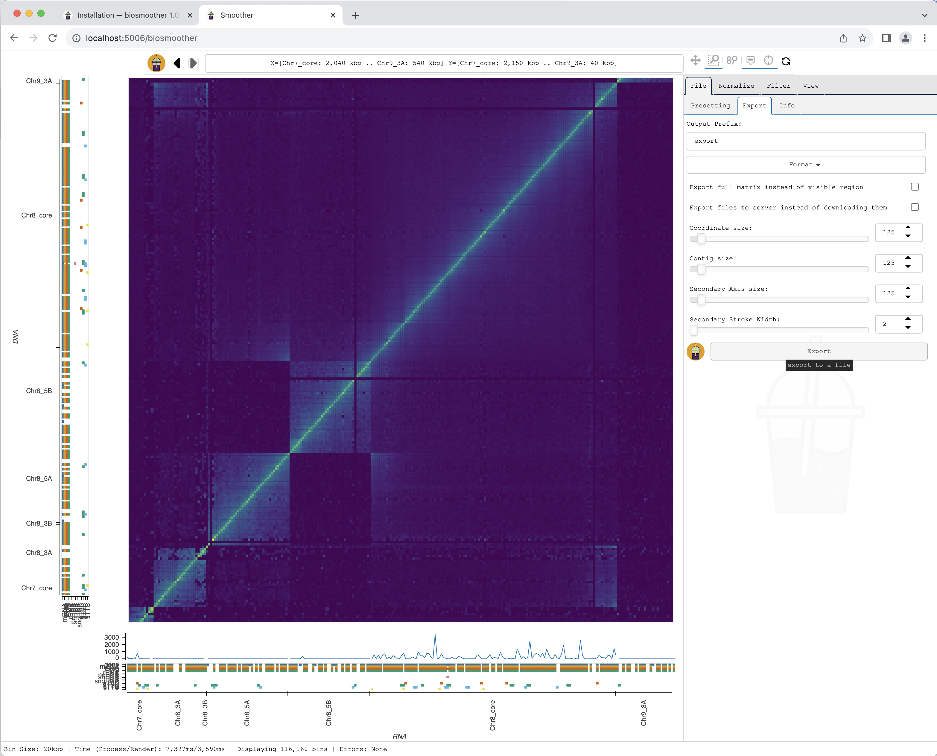
The picture file is saved.

Installation

Pip

The easiest way to install Smoother is via pip and conda

conda create -y -n smoother python=3.9 # create an environment for smoother
conda activate smoother # activate the environment
pip install biosmoother # install smoother and dependencies
conda install -y nodejs cairo # install non-pip dependencies

This will install biosmoother, the graphical user interface, and libbiosmoother, the backend behind the GUI and the command-line interface.

Compiling Smoother yourself

For installing Smoother via GitHub, run the following commands:

# create & activate an environment for smoother
conda create -y -n smoother python=3.9
conda activate smoother

# clone repository
git clone https://github.com/Siegel-Lab/BioSmoother.git
cd BioSmoother

# create the required conda environment
conda env create -f doncs_conf/dev_env_linux.yml

# install from local folder using pip
pip install -e .

While the pip installation will install the latest stable release, this type of installation will install the newest, possibly untested version. Note that this approach does still use pip to install the latest stable release of libBioSmoother and libSps, the two backend libraries behind Smoother. To also install these two libraries on your own, you will have to clone the respective repositories and install manually from them using the pip install -e . command. Then you can install Smoother using pip install -e . -no-deps to install Smoother without adjustments to the dependencies.

Supported operating systems and browsers

Smoother supports Linux, Windows, and MacOS. Specifically, we support:

macOS 10.9+ Intel 64Bit
macOS 10.9+ Apple Silicon 64Bit
Windows 64bit
manylinux2014 x86_64 (CentOS 7 & 8, Fedora 32+, Mageia 8+, openSUSE 15.3+, Photon OS 4.0+, Ubuntu 20.04+)
musllinux x86_64

Smoother has been tested on the latest versions of Firefox, Chrome, and Safari.

Command organization

Smoother has multiple subcommands, all of which interact with an index directory. An index contains the genome, its annotations, as well as the datasets to be analyzed and visualized. Each of the subcommands is designed to perform one specific task on the index. For example, there are the init and serve subcommands that can be called as follows:

biosmoother init ...
biosmoother serve ...

To see the main help page, run:

biosmoother -h

To see the help pages of the individual subcommands (e.g., for init), run:

biosmoother init -h

A complete list of subcommands can be found here. The following chapters explain how to use the subcommands for creating and interacting with indices.

Creating an index

All data to be analyzed and visualized on Smoother needs to be precomputed into an index. In the next chapters, we will explain how to initialize an index and fill it with data.

Initializing an index

Before an index can be filled with interactome data, we must set it up for a given reference genome. Generating an empty index is done using the init subcommand. The command outputs an index directory.

Let us create a new index for the Trypanosoma brucei genome.

If we have a .gff file, containing annotations for our genome, we must include this file right when creating the index:

biosmoother init my_index -a tryp_anno.gff

This command will create a folder called my_index.smoother_index. In all other subcommands, we can now use my_index to refer to this index. The tryp_anno.gff file must match the GFF specifications, and looks something like this:

##sequence-region Chr1 253215
##sequence-region Chr2 546247
Chr1   EuPathDB   gene   33710   34309   .   -   .   ID=Tb427_010006200.1;description=hypothetical protein / conserved
Chr2   EuPathDB   rRNA   1582219 1583848 .   -   .   ID=Tb427_000074200:rRNA;description=unspecified product

If, for some reason, we do not have a .gff file, we can also create an index without annotations However, then we need to supply a file containing the contig sizes of the genome:

biosmoother init my_index -c tryp.sizes

tryp.sizes is the file that contains the contig sizes of the genome. It looks something like this:

#contig_name contig_size
chr1 844108
chr2 882890

Important

Currently, we recommend Smoother only for genomes < 150Mbp in size, as indices might become very large (many hundreds of gigabytes) otherwise. The easiest way to reduce index size is to increase the base resolution of the index. For this, you can use the -d parameter of the init subcommand. The base resolution is the highest resolution that can be displayed, so do not set it lower than the resolutions you are interested in.

The full documentation of the init subcommand can be found here.

Adding replicates to an index

Adding data for a sample or replicate to an index is done with the repl subcommand. This requires an input pairs file containing the two-dimensional interactome matrix for the aligned reads. Preprocessing of the data and input pairs file generation are explained in detail in the next section.

The basic usage of the repl subcommand is as follows:

biosmoother repl my_index replicate_data replicate_name

Here, my_index is the index the data shall be added to, replicate_data is a file containing the actual data, and replicate_name is the displayname of that dataset in the user interface. There is a way to load gzipped (or similar) datafiles into Smoother using pipes:

zcat replicate_data.gz | biosmoother repl my_index - replicate_name

The full documentation of the repl subcommand can be found here.

Input format for the repl command

Smoother requires a whitespace (space or tab) delimited input pairs file containing the two-dimensional interactions. Each input pairs file contains the data for one sample or replicate to be analyzed and visualized. Each line in the file has the information for one interaction.

The default format for the input pairs file is compatible with the output from pairtools and corresponds to the following -C option for the repl subcommand: -C [readID] chr1 pos1 chr2 pos2 [strand1] [strand2] [.] [mapq1] [mapq2] [xa1] [xa2] [cnt]. Such a file would, for example, look something like this:

SRR7721318.88322997     chr1  284     chr1  4765    -       +       UU      0       0
SRR7721318.659929       chr1  294     chr1  366     +       -       UU      29      29      chr5,-1363,3S73M,2;chr11,+1132,73M3S,2;  chr6,-1131,2S74M,2;
# ...

Smoother also supports input files formatted as count matrices. A count matrix would look something like this:

chr1    1    chr1      1    123
chr1    1    chr1  10000     57

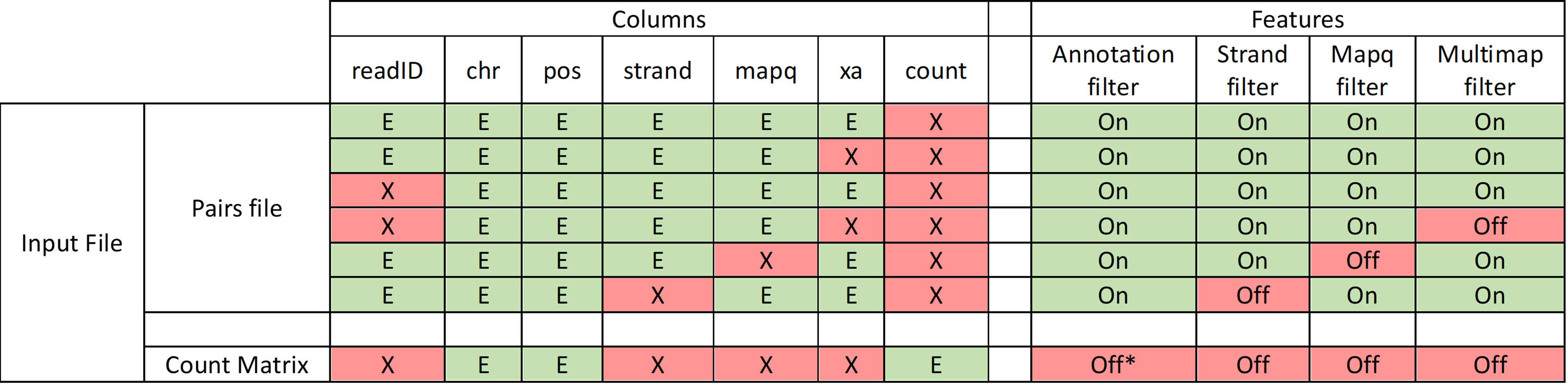
For this, please use the -C option chr1 pos1 chr2 pos2 cnt. However, it is important to note that the limited information in such files won’t allow Smoother to perform analyses at its full potential. Indeed, count matrices are already binned and thus the ‘pos’ columns correspond to the bin position. Hence, setting a smaller base resolution (with the -d option in the init subcommand) or using annotation filtering will not provide useful information and should be avoided, since the individual positions of reads have been lost by using a count matrix file. The functionalities of Smoother will be limited: 1) filtering by annotation will only be able to consider the bin locations instead of the actual read locations; 2) similarly, the base resolution of the heatmap will be limited by the bin size of the count matrix. For example, if the input pairs file has a bin size of 10 kbp, the heatmap will not be able to display a resolution higher than 10 kbp.

See the table below for a summary of filtering functionalities of Smoother depending on the input file format used to generate the index:

**Figure:** Summary of filtering functionalities of Smoother depending on the input file. E: column exists; X: column does not exist or contains a dummy value; On: filter is active; **Off**: filter is inactive; Off*: filter can be active, but it is uninformative because position is binned

The -C option accepts optional columns, indicated in squared brackets (e.g., with -C [readID] chr1 pos1 chr2 pos2 [strand1] [strand2], readId, strand1 and strand2 are optional). In this case, the input pairs file can contain rows with any of the following formats:

readID chr1 pos1 chr2 pos2 strand1 strand2
readID chr1 pos1 chr2 pos2 strand1
readID chr1 pos1 chr2 pos2
chr1 pos1 chr2 pos2

The following columns can be included in the input pairs file:

readID: sequencing ID for the read or read name
chr: chromosome (must be present in reference genome)
pos: position in basepairs
strand: DNA strand (+ or -)
.: column to ignore
mapq: mapping quality
xa: XA tag from BWA with secondary alignments with format (chr,pos,CIGAR,NM;)
cnt: read count frequency of row interaction.

Important

In the case of asymmetric data (like RNA-DNA interactome), 1 is the data displayed on the x-axis (columns) and 2 is the data displayed on the y-axis (rows). As default RNA is on the x-axis and DNA on the y-axis; however, this can be modified interactively after launching Smoother.

In the following subsections, we describe examples of the preprocessing workflow from raw demultiplexed fastq files to input pairs files for symmetric and asymmetric data sets.

Preprocessing data for the repl command

Symmetric data sets, such as Hi-C or Micro-C

The following steps are one example that can be followed to produce the input pairs files necessary to generate the index for Smoother from raw Hi-C data.

The raw read files are mapped to the reference genome using bwa mem.

bwa mem -t 8 -SP ${GENOME_NAME}.fna ${READ_FILE_1} ${READ_FILE_2}

Find ligation junctions and make pairs file using pairtools parse with the following options:

--drop-sam: drop the sam information
--min-mapq 0: do not filter by mapping quality
--add-columns mapq,XA: add columns for mapping quality and alternative alignments
--walks-policy mask: mask the walks (WW, XX, N*) in the pair_type column

pairtools parse --drop-sam --min-mapq 0 --add-columns mapq,XA --walks-policy mask ${GENOME_NAME}.sizes

Filter out the walks (WW, XX, N*) from the pairs file using pairtools select

pairtools select '(pair_type!="WW") and (pair_type!="XX") and not wildcard_match(pair_type, "N*")' {OUTPUT_PARSE}.pairs

Sort the output using pairtools sort

pairtools sort --nproc 8 {OUTPUT_SELECT}.pairs

Deduplicate the output using pairtools dedup

pairtools dedup {OUTPUT_SORT}.pairs

Generate the final pairs file that will be the input for generating Smoother index using pairtools split

pairtools split {OUTPUT_DEDUP}.pairs --output-pairs ${SAMPLE_NAME}.pairs.gz

Below, an example of some lines of a Hi-C input pairs file that can be used to generate the Smoother index.

## pairs format v1.0.0
#sorted: chr1-chr2-pos1-pos2
#shape: upper triangle
#genome_assembly: unknown
#chromsize: BES10_Tb427v10 41824
#chromsize: BES11_Tb427v10 66776
#chromsize: BES12_Tb427v10 48283
# ...
#columns: readID chrom1 pos1 chrom2 pos2 strand1 strand2 pair_type mapq1 mapq2 XA1 XA2
SRR7721318.37763890     BES10_Tb427v10  103     BES10_Tb427v10  4813    -       +       UU      0       0
SRR7721318.42386417     BES10_Tb427v10  184     BES10_Tb427v10  2446    +       -       UU      0       0
SRR7721318.659929       BES10_Tb427v10  294     BES10_Tb427v10  366     +       -       UU      29      29      unitig_172_Tb427v10,-1363,3S73M,2;BES12_Tb427v10,+1132,73M3S,2;BES12_Tb427v10,+1432,73M3S,2;unitig_172_Tb427v10,-1063,3S73M,2;  BES12_Tb427v10,-1131,2S74M,2;unitig_172_Tb427v10,+1063,74M2S,2;unitig_172_Tb427v10,+1363,74M2S,2;BES12_Tb427v10,-1431,2S74M,2;
# ...

Asymmetric data sets, such as RD-SPRITE, or RADICL-seq

The following steps are one example that can be followed to produce the input pairs files necessary to generate the index for Smoother from single-read raw RADICL-seq [1] data.

First round of extraction of the RNA and DNA tags from the chimeric reads containing the RADICL adapter sequence using tagdust. Here read1 will be RNA and read2 will be DNA.

tagdust -1 R:N -2 S:CTGCTGCTCCTTCCCTTTCCCCTTTTGGTCCGACGGTCCAAGTCAGCAGT -3 R:N -4 P:AGATCGGAAGAGCACACGTCTGAACTCCAGTCAC {READ_FILE} -t 38 -o {out1_R1D2}

Second round of extraction of the RNA and DNA tags from the chimeric reads containing the RADICL adapter sequence using tagdust. Here read1 will be DNA and read2 will be RNA.

tagdust -1 R:N -2 S:ACTGCTGACTTGGACCGTCGGACCAAAAGGGGAAAGGGAAGGAGCAGCAG -3 R:N -4 P:AGATCGGAAGAGCACACGTCTGAACTCCAGTCAC {out1_R1D2} -t 38 -o {out2_D1R2}

Concatenate two files with RNA reads using fastx_toolkit.

cat {out1_R1D2_READ1}.fq > {RNA}.fq
cat {out2_D1R2_READ2}.fq | fastx_reverse_complement -Q33 >> {RNA}.fq

Concatenate two files with DNA reads using fastx_toolkit.

cat {out1_R1D2_READ2}.fq | fastx_reverse_complement -Q33 >> {DNA}.fq
cat {out2_D1R2_READ1}.fq > {DNA}.fq

The RNA and DNA read files are mapped to the reference genome using bwa aln with -N parameter to keep the multimapping reads.

bwa aln -N ${GENOME_NAME}.fna {RNA}.fq > {RNA}.sai
bwa aln -N ${GENOME_NAME}.fna {DNA}.fq > {DNA}.sai

Convert the output from the alignment to SAM format with a value for the -n parameter high enough to keep all interesting multimapping reads.

bwa samse -n 60 ${GENOME_NAME}.fna {RNA}.sai {RNA}.fq > {RNA}.sam
bwa samse -n 60 ${GENOME_NAME}.fna {DNA}.sai {DNA}.fq > {DNA}.sam

Generate tab-separated text files for RNA and for DNA with the information from the SAM files and adding dummy values (notag) if there is no XA tag.

cat {RNA}.sam | awk -F '\t' 'BEGIN {OFS="\t";ORS=""} {if ($1 ~ !/^@/ && $3 ~ !/*/) {print $3,$4,$1,$5; for(i=12;i<=NF;i+=1) if ($i ~ /^XA:Z:/) print "",$i; print "\n"}}' | awk -F '\t' 'BEGIN {OFS="\t";ORS=""} {print $1,$2,$3,$4; if(NF<5) print "\tnotag"; else print "",$5; print "\n"}' >> {RNA}
cat {DNA}.sam | awk -F '\t' 'BEGIN {OFS="\t";ORS=""} {if ($1 ~ !/^@/ && $3 ~ !/*/) {print $3,$4,$1,$5; for(i=12;i<=NF;i+=1) if ($i ~ /^XA:Z:/) print "",$i; print "\n"}}' | awk -F '\t' 'BEGIN {OFS="\t";ORS=""} {print $1,$2,$3,$4; if(NF<5) print "\tnotag"; else print "",$5; print "\n"}' >> {DNA}

Sort the RNA and DNA tab-separated text files.

sort -k1,1 -k2,2n {RNA} > {RNA_k1k2}
sort -k1,1 -k2,2n {DNA} > {DNA_k1k2}
sort -k3,3 {RNA_k1k2} > {RNA_k3}
sort -k3,3 {DNA_k1k2} > {DNA_k3}

Merge the RNA and DNA files based on the sequencing ID (column 3) to generate a single interactome file.

join -j 3 {RNA_k3} {DNA_k3} | awk 'BEGIN{OFS="\t"}{print $2,$3,$1,$4,$5,$6,$7,$1,$8,$9}' > {R_D}

Below, an example of some lines of a RADICL-seq input pairs file that can be used to generate the Smoother index.

SRR9201799.1 NC_000077.7 108902883 NC_000079.7 9361584 0 37 XA:Z:NC_000079.7,-97327088,27M,0;NC_000075.7,-3258605,27M,1;NC_000086.8,+13535333,27M,2; notag
SRR9201799.10 NC_000075.7 46047334 NC_000075.7 45133248 0 37 notag notag
SRR9201799.100 NC_000078.7 115363700 NC_000084.7 55062439 0 37 notag notag
SRR9201799.1000 NC_000084.7 16977496 NC_000074.7 35058114 0 37 XA:Z:NC_000072.7,+128816081,26M,0;NC_000072.7,-128737045,26M,0;NC_000072.7,-128775829,26M,0;NC_000082.7,+32868030,26M,0;NC_000068.8,+27291980,26M,0; notag
SRR9201799.10000 NC_000083.7 68621840 NC_000070.7 132889911 25 37 XA:Z:NC_000078.7,+35879646,10M1I16M,2; notag
SRR9201799.100000 NC_000079.7 97327088 NC_000077.7 115303050 0 23 XA:Z:NC_000077.7,-108902883,27M,0;NC_000075.7,-3258605,27M,1;NC_000086.8,+13535333,27M,2; XA:Z:NC_000086.8,+43444132,25M,2;
SRR9201799.1000000 NC_000068.8 98497428 NC_000075.7 98504289 0 37 notag notag
# ...

Adding tracks to an index

Adding unidimensional data to an index is done with the track subcommand. Such unidimensional data is displayed as coverage tracks next to the main heatmap. The track subcommand thus allows overlaying RNA-seq, ChIP-seq, ATAC-seq or other datasets to the heatmap. Input file generation are explained in detail in the next section.

The basic usage of the track subcommand is as follows:

biosmoother track my_index track_data track_name

Here, my_index is the index the data shall be added to, track_data is a file containing the actual data, and track_name is the displayname of that dataset in the user interface. There is a way to load gzipped (or similar) datafiles into Smoother using pipes:

zcat track_data.gz | biosmoother repl my_index - track_name

The full documentation of the track subcommand can be found here.

Input format for the track command

Smoother requires a whitespace (space or tab) delimited input coverage file for the secondary data to be loaded with the track subcommand.

The default format for the input coverage file corresponds to the following -C option for the track subcommand: -C [readID] chr pos [strand] [mapq] [xa] [cnt].

The input coverage file can be generated from a .bed or .sam file from the secondary data set. As an example, the input coverage file can be directly generated from the bwa mem .sam output using the following command:

cat alignments.sam | awk '!/^#|^@/ {print $1, $3, $4, $2 % 16 == 0 ? "+" :"-", $5, $12}' OFS="\t" > coverage

Alternativeley, a bigWig file can be loaded using the bigWigToBedGraph tool:

bigWigToBedGraph input_file.bg | awk ‘{$4=int($4*10000); print $0}’ | biosmoother repl - repl_name -C chr pos . cnt

Using the graphical interface

Launching the graphical interface

Launching the Smoother interface for an existing index is done with the serve subcommand. If an index has already been launched before, the session will be restored with the parameters of the last session, as they are saved in the session.json file in the index directory. The Smoothers interface makes use of the Bokeh library. For example, this is how we would launch an index called my_index:

biosmoother serve my_index -show

The full documentation of the serve subcommand can be found here.

Port forwarding on a server that uses slurm

Smoother is set up to be run on a server with the Slurm Workload Manager.

For this, you need to forward a port from the compute node over the master node to your local computer. This port forwarding allows you to reach the Smoother application with the web browser of your local computer even though it is running on one of the client nodes on the server. First, log into the main node of the server with ssh port forwarding. The default port that needs to be forwarded is 5009; this requires the following login command:

ssh -L 5009:localhost:5009 -t your_user_name@your_server

Now, any internet-traffic that is using the port 5009 is directed to the server you just logged in to. Then, queue into one of the client nodes on the server by:

srun --pty bash

Now, forward the port from the master node to the client node that you just lokgged in to:

sshfwd="ssh -fNR 5009:localhost:5009 ${SLURM_JOB_USER}@${SLURM_LAUNCH_NODE_IPADDR}"; trap 'kill $(ps h -o pid -C "$sshfwd")' EXIT; $sshfwd

This command will ask you for your password. After entering it, the port forwarding is set up and you can launch Smoother on the client node. The command to launch Smoother is:

conda activate smoother # activate the conda environment if necessary
biosmoother serve my_index --port 5009

The command will print an url on your terminal. Follow this url with any web browser to open Smoother on the server. To allow multiple users to use Smoother at the same time, you can use a different port for each user, replacing all 5009 in the above commands with 5010, 5011, and so on.

Setting up a webserver with Smoother

Since Smoother is a web application, it can be set up as a webserver. This allows multiple users to access Smoother at the same time. To do this, you can use the --keep_alive, and --no_save options, so that Smoother does not shutdown once one user leaves and does not save the changes made by one user for the next user. To allow other machines connecting to the server, you have to configure the --allow-websocket-origin option. For example, to allow connections from any machine, you can use the following command: --allow-websocket-origin=*.

Overview of Smoother’s interface

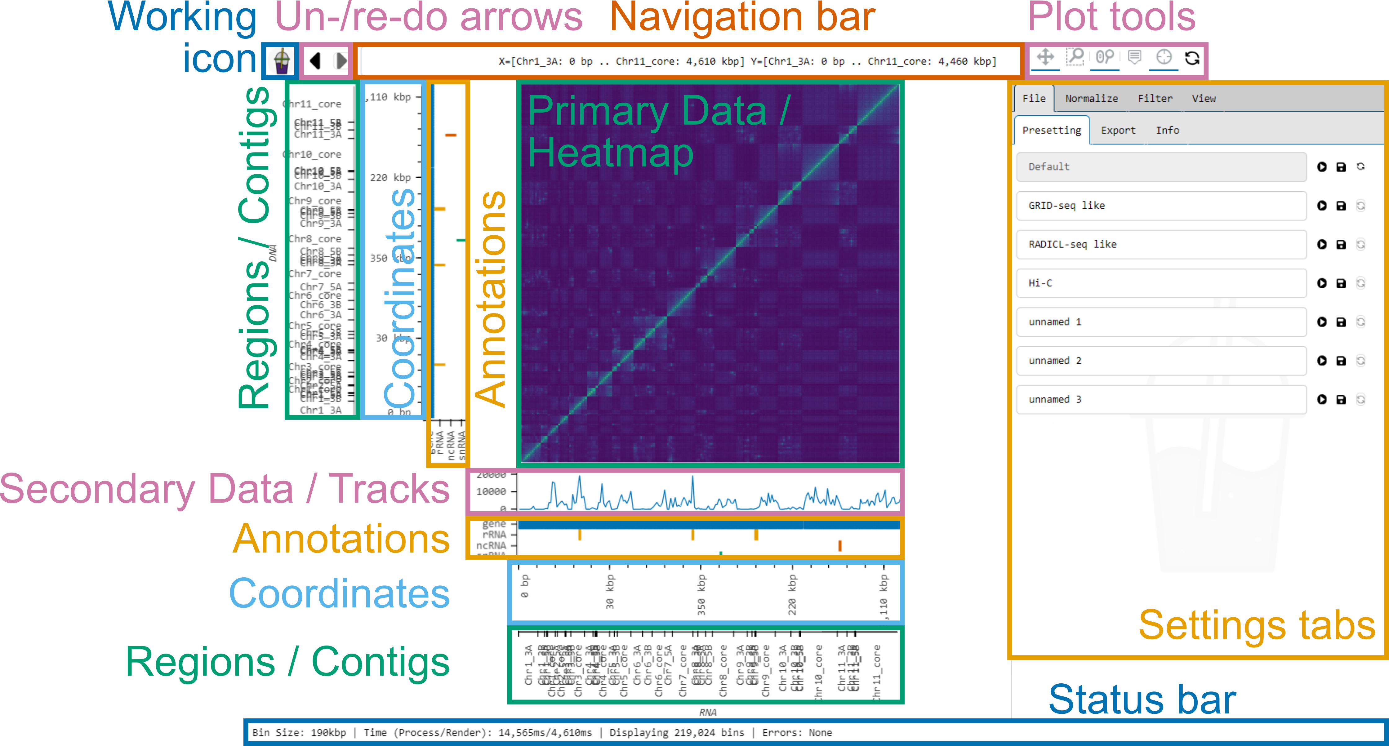
**Figure:** Smoothers' Panels labeled by name.

Smoother’s interface consists of several panels:

Working icon: Displays the current status.
Un-/re-do arrows: Click to undo or redo changes.
Navigation bar: Displays the currently visible region and allows to jump to a region of interest.
Plot tools: Allows toggling ways to interact with the plots.
Primary data: Displays the heatmap.
Secondary data: Displays the coverage tracks.
Annotations panel: Displays the annotations.
Coordinate axis: Displays the coordinates within the contigs.
Regions axis: Displays the contigs.
Status bar: Displays the current status of Smoother.
Settings tabs: Allows changing the on-the-fly analysis parameters of Smoother.

Panels can be shown and hidden using the View->Panels Show / Hide dropdown menu. The Annotation and the Secondary data panel hide themselves automatically if they do not contain data.

Smoothers status can be one of three things. Working: , error: , waiting: .

On the right-hand side of the interface, there are several tabs with buttons and sliders. These can be used to change several analysis parameters on-the-fly.

Navigation on Smoother

Navigation on Smoother is controlled by the panels on the top. On the top left, the two arrows allow undoing and redoing changes. On the top central panel, the coordinates for the visible region are displayed and can be modified to navigate to a region of interest, as described in the navigation bar chapter below. On the top right, several tools to interact with the plots can be activated (see the plot tools chapter below).

Plot tools

The control panel on the top right corner has the following buttons from left to right: Pan, Box zoom, Wheel zoom, Hover, Crosshair, and Reset.

Pan enables navigation by clicking and dragging in the plots.
Box zoom allows to zoom into a region of interest by selecting the region with a box.
Wheel zoom enables zooming in and out by scrolling.
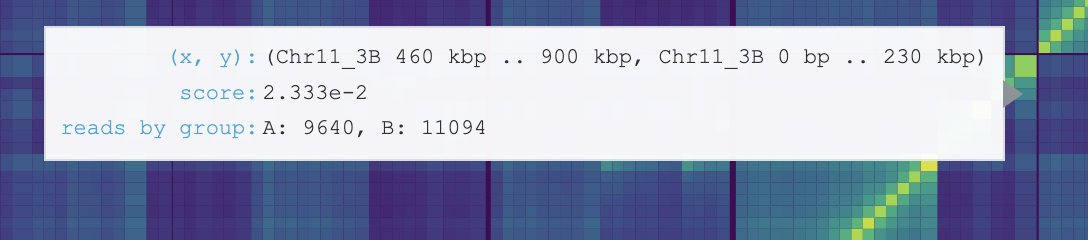
Hover displays information for the genomic coordinates, interaction score, and reads by group for the current bin of the heatmap. Hover also displays information of the name and colour of displayed coverage tracks and the scores for the current bins in the coverage track.
Crosshair highlights the row and column coordinates of the current location.
Reset resets the heatmap to default settings.

**Left:** Hovering over a bin in the heatmap with the Hover tool enabled.

The Navigation bar

The Navigation bar on the top centre of the graphical interface displays the currently visible region, every time Smoother renders a new heatmap. However, you can also input a location into the bar and Smoother will jump to that location in the heatmap.

For this, click into the Navigation bar and replace the text with the region you want to jump to. (A simple way to replace all text in the bar is clicking into it and hitting control-a, then typing the new location).

The bar accepts the following syntax and various short forms of if:

X=[chrX1: 10 kbp .. chrX2: 100 kbp] Y=[chrY1: 20 kbp .. chrY2: 200 kbp]

Here, chrX1: 10 kbp is the start horizontal location, while chrX2: 100 kbp is the horizontal end location. The same goes for chrY1 and chrY2 as the vertical start and end locations. Several units are accepted: bp, kbp, and Mbp. The square brackets around the coordinates of either axis are optional. Note that two dots .. are used to delimitate the start and end locations on an axis; this is essential, you cannot use one, three or more dots.

If you want to merely change the range of the x-axis, you can omit the Y=[...] portion of the command (vice versa for the y-axis).

X=[chrX1: 10 kbp .. chrX2: 100 kbp]

If you want to change both axes to the same region, simply drop the X= and Y=

chr1: 10 kbp .. chr2: 100 kbp

If the entire contig shall be visible, coordinates can be omitted:

chr1 .. chr2

Here the heatmap would include chr1 and chr2 fully: I.e., start at the beginning of chr1 and end at the end off chr2. If you want to visualize only one contig you can use this:

chr1

Let’s say you want to display chr1, with 100 kbp of extra space around it, you could use the following command:

chr1: +- 100 kbp

Instead of adding extra space around the entire contig, one can also pick a specific position. For example, one could show the region from 400 kbp to 600 kbp on chr1.

chr1: 500 kbp +- 100 kbp

Further, showing the region from 100 kb to 200 kbp on chr1 is also possible:

chr1: 100 kbp .. 200 kbp

Negative coordinates are allowed, the following command will show a 200 kbp region centered around the start of chr1:

chr1: -100 kbp .. 100 kbp

Capitalization does not matter for all inputs to the Navigation bar.

Hint

Inputting a * into the Navigation bar will make the full heatmap visible.

The Status bar

The status bar displays a bunch of information about the current state of Smoother.

Bin size: First, the size of the currently visible bins is shown. If bins are squared, one number is given, while for rectangular bins the size is given as width x height.
Times: Next, Smoother displays the time it took to process and render the currently visible heatmap.
Number of bins: Then, the total number of bins is shown.
Errors: Finally, if there are any errors, they are displayed here.

If you trigger Smoother to re-render the heatmap, the status bar will display that Smoother is rendering and the reason why.

The File tab

In the File tab of Smoother, there are three subtabs: ->Presetting, ->Export, and ->Info.

The Presetting subtab

File->Presetting allows performing analysis with predetermined settings.

A presetting can be applied using the 'play' button ().

Three analyses are already preconfigured and available on Smoother for doing normalizations as in GRID-seq [2] [3] , RADICL-seq [1], as well as one for Hi-C data.

It is also possible to save the current settings configured on Smoother as a new presetting, using the 'floppy disk' button (). Every presetting can be reset to factory default, using the 'arrow' button ().

The Default presetting contains the parameters that are applied to an index when first loading it. Presettings only contain parameters that are independent of the data of the index. For example, assigning primary datasets into pool A or B, depends on the datasets that are loaded in the index and thus cannot be saved as a presetting. The type of normalization that is applied on the other hand is saved as a presetting, since it is independent of the data. Specifically, all parameters that are in the ‘Settings’ group are saved in a presetting.

The Export subtab

File->Export allows to save the interactome data with the settings of the current session either as a TSV text file or as a picture in SVG or PNG format. It is possible to export only the visible region or the full heatmap using the export full matrix instead of visible region checkbox.

The path for the exported files can be specified on the Output Prefix box.
The format can be selected clicking on the Format dropdown.
If files need to be exported to the server instead of being downloaded, it is possible to check the box Export files to server instead of downloading them .
The pixel size for coordinates, contigs, secondary axis and stroke width can be selected prior to export.
When saving as TSV, 3 files are saved, one for the interactome, and one for each axis.

Exporting with settings thus allows to save interactome data with all active filters, normalization, comparison between groups, and even virtual 4C analyses.

The Info subtab

File->Info provides a log of Smoother processes, which are also displayed on the command line.

Download current session allows exporting the metadata by downloading all the parameters of the current session.
upload session allows setting all the parameters of the current session by uploading a file.

The Normalize tab

In the Normalize tab of Smoother, there are three subtabs: ->Primary, ->Dist. Dep. Dec., and ->Ploidy. It is possible to perform one Normalize->Primary normalization and also perform the ->Dist. Dep. Dec. and ->Ploidy correction.

The Primary subtab

Several normalizations are available in the Normalize->Primary subtab to normalize the heatmap or the coverage track. Using the Normalize heatmap by dropdown, the heatmap and coverage can be normalized by Reads per million or Reads per thousand on the visible region. It is worth noting that the visible color changes automatically on screen (can be modified on the View tab) and thus the heatmap might not change visually between No normalization, Reads per million, or Reads per thousand. However, the values of the bins do change, and they are what is relevant for exporting the TSV text file for downstream analyses. The coverage can also be normalized by Reads per million base pairs and Reads per thousand base pairs, so that normalization can be done by the size of the bin, indicating the density of reads in one million or thousand base pairs squared.

The other normalizations available for heatmap on Smoother are performed with a sampling strategy that also considers some bins outside of the visible area for normalization [5] . The normalizations available for the heatmap (also in the Normalize heatmap by dropdown) based on the sampling strategy are Binomial test [1] , Iterative correction [4] and Associated slices [2] [3] . The number of samples taken outside the visible region can be modified on the slider bar Number of samples to ensure the lowest deviation from normalizing to the entire heatmap [5] .

Hint

If it is essential that the normalization runs on the entire heatmap it is possible to 1) export the normalized interactome (whole heatmap), and 2) generate a new index on Smoother. This will allow zooming in to regions normalized to the entire heatmap.

The Binomial test and Associated slices normalizations are implemented for asymmetric RNA-DNA interactome data and Iterative correction is the default normalization for Hi-C data.

Binomial test normalization

Binomial test: determines statistical significance of each bin over the genome-wide coverage of the interacting RNA. A slider bar allows to modify the pAccept for binomial test which is the value at which the p-value is accepted as significant. It is possible to select the option to display coverage of the normalization in the secondary data panel using the Display coverage as secondary data checkbox. It is also possible to change the axis in which the normalization is performed (Apply binomial test to columns), by default this normalization is performed row-wise but if the box is checked the normalization is performed column-wise.

**Figure:** Normalizing RNA-DNA interactome data by Binomial test.

Associated slices normalization

Associated slices: normalizes each bin by the sum of trans chromatin-associated slices of the interacting RNA. First, chromatin-associated slices need to be determined. For this, we compute the Average RNA reads per kb and the Maximal DNA reads in a bin for a set of slices. You can adjust the Number of samples taken, using the so-named slider. Slices are chosen from a type of annotation, where the vertical size of bins is determined by the individual annotations. The specific Annotation type can be picked using a dropdown button. For the Maximal DNA reads, horizontal bin size can be adjusted using the Section size max coverage slider. Average RNA reads are always normalized to 1 kb bins. Slices are considered as chromatin-associated if they fall into the ranges set by the RNA reads per kbp bounds and Maximal DNA reads in bin bounds sliders. To visualize the effects of these bounds, two plots show the distribution of the Average RNA reads per kb and the Maximal DNA reads in a bin for the selected slices. Grey dots indicate slices that are filtered out. Finally, bins are normalized by the trans coverage of the slices. You can display this coverage using the Display background as secondary data checkbox. (For comprehensive computational explanation of this normalization see the Smoother manuscript [5] and the GRID-seq publication [2] [#grid_seq2]*). GRID-seq [#grid_seq1]* [3] uses this normalization in combination with filtering out reads that do not overlap genes on their RNA read (see the Filter->Annotations tab).

It is possible to change the axis in which the normalization is performed using the Compute background for columns checkbox, by default this normalization is performed column-wise but if the box is unchecked the normalization is performed row-wise. A checkbox allows to choose whether to use the intersection of chromatin-associated slices between datasets as background, otherwise the union of slices is used. This is relevant because the normalization is done separately on the datasets, but to make the normalization match between the datasets, the chromatin-associated slices need to match. The Ignore cis interactions box also allows to either ignore or consider cis interactions (within same contig).

**Figure:** Normalizing RNA-DNA interactome data by Associated Slices.

Iterative correction normalization

Iterative correction (IC): equalizes the visibility of the heatmap by making its column and row sums equal to a constant value. A bias value is computed for every slice (column and row) and IC normalization of the bins is performed by multiplying each bin by the biases of its column and row. It is possible to filter out slices with more than the given percentage of empty bins using the filter out slices with too many empty bins [%] slider. A checkbox allows to Show bias as tracks in the secondary data panels. It is possible to use only the visible region to compute the IC by checking the Local IC box. The Mad Max filter slider allows to filter out bins for which the log marginal sum is lower than the given value. One slider bar allows to set the threshold for Minimal number of non-zero bins per slice, removing slices with less bins. Another slider can be used to ignore the n closest bins to the diagonal for bias computation (Ignore first n bins next to the diagonal).

**Figure:** Normalizing 3C data by ICing.

The Dist. Dep. Dec. subtab

The Normalize->Dist. Dep. Dec. subtab allows to perform a distance dependent decay normalization by selecting the checkbox Normalize Primary data. The distance dependent decay is computed with the mean of the value for all the bins at the same distance from the diagonal for the current contig. The normalization divides each bin by this mean. The mean can be displayed on a plot below by checking the box Display. On the plot, each line represents a bin with the beginning being the top left corner and the end being the bottom right corner of the bin. It is important to consider that the further away from the diagonal a bin is in a contig, the less bins it has at the same distance (or none for the corner bin). A slider allows to modify the minimum and maximum number of samples to compute for each diagonal. The top and bottom percentiles of samples can be excluded from the normalization with the Percentile of samples to keep (%) slider.

**Figure:** Normalizing 3C data by distance dependent decay.

Hint

Distance Dependent decay normalization can be applied on top of a primary normalization and/or the ploidy correction.

The Ploidy subtab

Many organisms are aneuploid or comprise chromosomes where some regions are homozygous and some are highly heterozygous. While with a “normal” diploid organism each contig of the organism’s assembly corresponds to two physical chromosomes of a set, aneuploid organisms harbor an abnormal number of chromosomes. For aneuploid organisms, some contigs might correspond to one (set of) physical chromosome(s), while others correspond to two or more. The same situation occurs with varying zygosity. For example, in some organisms, the chromosome sets have homozygous central regions (cores) flanked by heterozygous peripheral regions. While the cores would be collapsed into one contig in their genome assembly, the peripheral regions would be assembled separately. Therefore, the core contigs would correspond to two physical regions, while each of the peripheral contigs would correspond to one physical region. We call such contigs misrepresented.

The Normalize->Ploidy tab allows correcting for such misrepresentation. First, a .ploidy file must be uploaded using the replace ploidy file button. The format of .ploidy files is described in the Ploidy input format chapter below. To perform the ploidy correction do correct must be checked and checking use ploidy corrected contigs will trigger Smoother to use the order of contigs from the ploidy corrected file instead of the genome sizes file. The correction considers n-ploid contigs as n instances and interactions are divided evenly among the instances of the contigs. The correction has several options that can be selected on the following checkboxes:

Remove inter-contig, intra-instance interactions will remove interactions between two different instances of the same contig.
Keep interactions from contig-pairs that are in the same group will keep interactions if they belong to the same contig-groups which are defined in the ploidy file (see example on top).
Keep interactions from contig-pairs that never occur in the same group will keep interactions only if they don’t belong to the same contig-groups which are defined in the ploidy file
Remove interactions that are not explicitly kept by the options above

An example that requires ploidy correction is T. brucei: Its genome is organized in diploid chromosomes, with homozygous core regions and heterozygous subtelomeric regions. In the genome assembly, such a chromosome (e.g., chromosome 1) is composed of five contigs: two contigs for the 3’ subtelomere ( 3’A_chr1 and 3'B_chr1 ), one contig for the core (core_chr1), and two contigs for the 5' subtelomere (5'A_chr1 and 5'B_chr1). In this case, ploidy correction works by defining the following two groups: 3'A_chr1-coreA_chr1-5'A_chr1, 3'B_chr1-coreB_chr1-5'B_chr1, where coreA_chr1 and coreB_chr1 are two instances of the core_chr1 contig. As with intra-contig interactions, we assume intra-group interactions to take prevalence. In detail, for every contig pair where at least one contig has multiple instances, interactions are split among the pair's instances that are within a group, if at least one pair-instance is within a group. Otherwise, interactions are split among all instances. Hence, interactions occurring between 5'A_chr1 and core_chr1 would be assigned to the 5'A_chr1-coreA_chr1 instance and not to 5'A_chr1-coreB_chr1. Furthermore, interactions between core_chr1 and a heterozygous contig 5'A_chr2 would be evenly distributed between coreA_chr1-5'A_chr2 and coreB_chr1-5'A_chr2.

Hint

Ploidy correction can be applied on top of other normalizations.

Ploidy input format

We have designed a custom format for correcting an index for ploidy. This format is a tab-separated text file with two columns: source and destination. All lines starting with a # are ignored. Entries in the source column contain the contig names of the genome assembly, exactly as they were specified in the .sizes file given to the init command. Entries in the destination column contain the contig names of the genome assembly, as they should be displayed in the user interface.

Correcting for ploidy is done by listing the same source for multiple destination columns. In the example below, we have the contigs Chr1_core, Chr1_5A, Chr1_3A, Chr1_5B, and Chr1_3B which express a chromosome set with a homozygous core but heterozygous subtelomeric regions. We correct for Chr1_core having 2 physical copies by listing Chr1_core as the source for Chr1_coreA and Chr1_coreB. All other contigs having only one physical copy and do not need to be corrected.

Finally, there are --- lines in the ploidy file. These lines are used to delimitate groups. The purpose of groups is to limit the correction to within the groups. For example: We want interactions between Chr1_core and Chr1_5A to occur in Chr1_coreA-Chr1_5A, not in Chr1_coreB-Chr1_5A. We achieve this by placing Chr1_coreA and Chr1_5A in the same group.

Interactions between Chr2_5A and Chr1_core, will be split evenly between Chr2_5A-Chr1_coreA and Chr2_5A-Chr1_coreB, since Chr2_5A and Chr1_core are never in the same group.

Here is an example ploidy file:

#columns: Source Destination
# chr1A
Chr1_5A     Chr1_5A
Chr1_core   Chr1_coreA
Chr1_3A     Chr1_3A
---
# chr1B
Chr1_5B     Chr1_5B
Chr1_core   Chr1_coreB
Chr1_3B     Chr1_3B
---
# chr2A
Chr2_5A     Chr2_5A
Chr2_core   Chr2_coreA
Chr2_3A     Chr2_3A

The Filter tab

In the Filter tab of Smoother, there are four subtabs: ->Datapools, ->Mapping, ->Coordinates, and ->Annotations.

The Datapools subtab

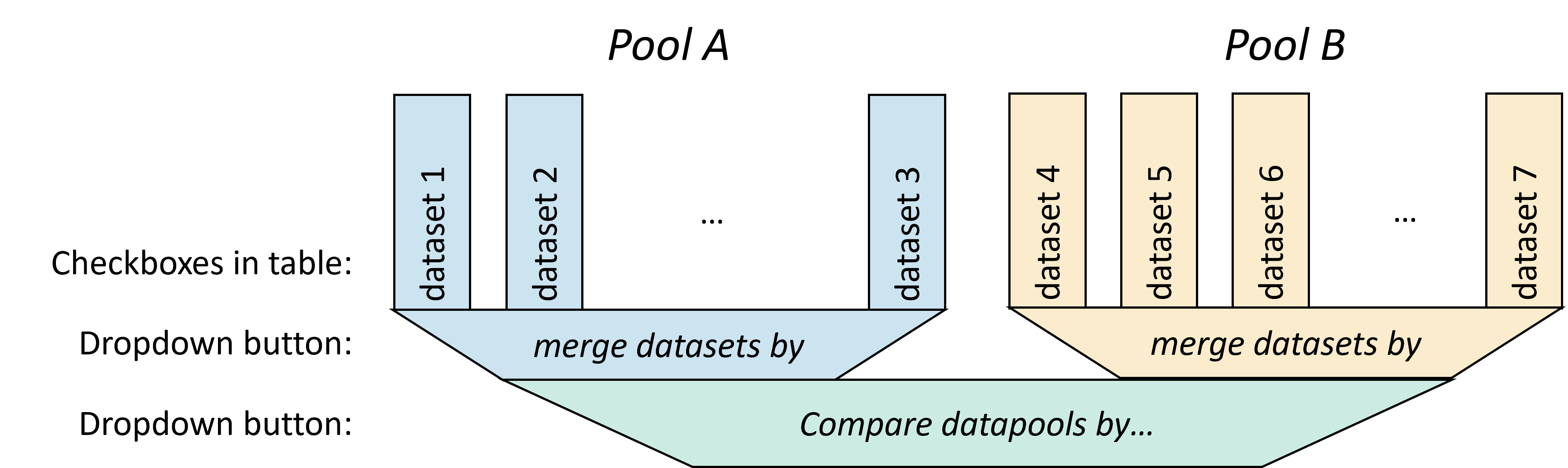
Filter->Datapools allows to define the group or condition for every sample and the type of comparison and representation that should be performed among the samples. The Primary Datapools table allows to distribute the samples with interactome data displayed on the heatmap in groups by assigning samples to different pools. The Secondary Datapools table allows to select the axis in which the secondary data panel with unidimensional data should be displayed. A dropdown menu allows to Merge datasets belonging to the same datapool group by several operations: sum, minimum, difference and mean. A second dropdown menu Compare datapools by enables the selection of options to display the combined datapools: sum, show first group a, show first group b, substract, difference, divide, minimum and maximum.

**Figure:** A visual representation of how datasets are first combined into two datapools, before these datapools are combined in turn.

**Figure:** Using the *subtract* option of the *Compare datapools by* dropdown menu, images like this can be generated.

The Mapping subtab

Filter->Mapping allows filtering interactions by mapping quality scores of their reads. The mapping quality score represents the confidence of the aligner for the correctness of each alignment. The highest possible score is 254 and the lowest is 0. The bounds and thresholds that can be used to filter the reads correspond to those listed as -m option when running the init command to generate the index. As default the lower bounds are 0, 3 and 30; and the upper bounds are 3, 30 and 255. The bounds for this filter can be selected on the dropdown menus Mapping Quality: Lower Bound and Mapping Quality: Upper Bound.

**Figure:** Filtering out reads with low mapping qualities.

One key functionality of Smoother is the possibility to analyze regions of high homology and repeats as multimapping reads can be kept given a lower bound of 0 in the Mapping Quality: Lower Bound. To do so, the smallest possible rectangle enclosing all possible alignments for a multimapping read is computed. A dropdown menu allows to select the preferred option to deal with the multimapping reads (MMR) in the scenarios that these rectangles are confined within a bin or overlap more than a bin:

Count MMR if all mapping loci are within the same bin. This is the default option.
Count MMR if mapping loci minimum bounding-box overlaps bin. It is important noticing that this will overrepresent the multimapping read as it will be displayed in more than a bin.
Count MMR if bottom left mapping loci is within a bin. This option allows displaying MMR if the bottom left mapping loci from the bounding-box is in the same bin even if mapping loci on top right corner fall outside the bin. This option only considers the bottom left-most mapping loci, ignoring all others.
Count MMR if top right mapping loci is within a bin. This option allows displaying MMR if the top right mapping loci from the bounding-box is in the same bin even if mapping loci on bottom left corner fall outside the bin.
Ignore MMRs. Multi-mapping reads are excluded from the analysis.
Count MMR if all mapping loci are within the same bin and ignore non-MMRs. This option allows analysis only of multimapping reads that are enclosed in a bin. This option can be useful for exploratory purposes.
Count MMR if mapping loci minimum bounding-box overlaps bin and ignore non-MMRs. This option allows analysis of multimapping reads that are not enclosed in a bin. This option can be useful for exploratory purposes.

A checkbox allows to show multimapping reads with incomplete mapping loci lists, which correspond to those that have too many mapping locations to be reported with the given maximum when running the mapping. When running the alignment with bwa, the maximum number of alignments to output in the XA tag can be predetermined with the -n option for the bwa samse command, and if there are more hits than the -n value, the XA tag is not written. It is important to notice that displaying these multi-mappers might introduce noise to the heatmap.

**Figure:** Filtering out multimapping reads that overlap multiple bins.

The Directionality dropdown menu allows choosing whether to display interactions for which interaction partners map to any or a particular strand. The options are the following:

Count pairs where reads map to any strand
Count pairs where reads map to the same strand
Count pairs where reads map to opposite strands
Count pairs where reads map to the forward strand
Count pairs where reads map to the reverse strand

The Coordinates subtab

Filter->Coordinates allows filtering the regions displayed on the heatmap.

In the Active contigs table, the contigs from the reference genome to be displayed on the two axes from the heatmap can be selected by tick boxes. The order in which the contigs are displayed can be modified by moving the contig names up or down using the arrows.

The dropdown Symmetry gives four options to filter interactions by symmetry:

Show all interactions displays all interactions from the input pairs file which might not be redundant if interactions only appear once and thus might only display on one of the two triangles on the sides of the diagonal.
Only show symmetric interactions displays only symmetric interactions on asymmetric matrices (RNA-DNA) or on redundant DNA-DNA heatmaps. It is worth noting, that for non-redundant Hi-C heatmaps, this option would only show the diagonal.
Only show asymmetric interactions displays only asymmetric interactions and is useful for asymmetric matrices (RNA-DNA).
Mirror interactions to be symmetric allows showing interactions on the two sides of the diagonal for non-redundant Hi-C matrices. Should be used for upper-triangle matrices (see the -u parameter of the init command.).

The Minimum Distance from Diagonal slider allows setting a minimal Manhattan distance by filtering out bins that are closer to the diagonal than the set value in kbp.

Annotation coordinate system

The dropdown Annotation Coordinate System menu allows to select the annotation type to use as the annotation coordinates. Two tick boxes allow activating the coordinate system for rows and/or columns. If this coordinate system is activate, the whitespace between the annotations is removed. I.e. the bins are placed only on the annotations. This will shrink down the size of the heatmap. Only annotations that have been listed on the -f option when running the init command to generate the index are available, as default the filterable annotation is gene.

When zooming in at one annotation, there are multiple ways to place bins. The dropdown Multiple Bins for Annotation let’s you choose to:

Stretch one bin over entire annotation: Places one bin per annotation. Since annotations might have different sizes, this will result in bins of different sizes (visually and on the genome).
Show several bins for the annotation: Place as many bins as you can fit into the annotation. This will result in bins of the same sizes (visually ad on the genome).
Make all annotations size 1: Compress all annotations to be of size 1, then place one bin per annotation. This will result in bins that are visually of the same size, however, on the genome bins will still cover the uncompressed annotations and therefore have different sizes.

Prioritized annotation coordinate system

When picking using the annotation coordinate system, it is crucial to filter out reads that do not overlap the chosen annotation type. Let’s say we use ‘gene’ coordinates on the x-axis. Then, each column of the heatmap corresponds to one gene. At least at at the most zoomed in level. However, when zooming out, Smoother has to keep the number of bins that are visible on screen roughly constent. Hence, at some points it will have t display two ore more neighboring genes in one column. This is all good and fine as long these neighboring genes are also neighbors in the genome. However, most likely, they are not. There will be some gap in between the genes. When grouping the genes together into one column we hence have to remove the reads that fall into these gaps. The best way to do this is using the Annotation filter, to remove all genes that do not overlap a gene on the x-axis. In fact, this filter is automatically activated when using the annotation coordinate system. However, this filter cannot be used for all annotation types. It is only computed for a handful of annotation types that were specified when running the init command to generate the index. So, what do we do if we do not want to recompute the whole index just to try out annotation coordinates.

We came up with a few options: The dropdown Multiple Annotations in Bin gives four options to deal with bins that comprise multiple annotations:

Combine region from first to last annotation: This is the option for the annotation filtering.
Increase number of bins to match number of annotations (might be slow): This will obviously fix our problem, but when looking at large regions, this will be very slow since too many bins will have to be computed.
Use first annotation in Bin: Counting only the first annotation in the bin will make sure that we do not count any reads that fall into the gap between the genes. However, while moving around or zooming, the first annotation of a bin will change. Hence, the heatmap will appear to ‘sparkle’. While moving around, every now and then an annotation with a strong interation will be the first in a bin, lighting up in the heatmap.
Use one prioritized annotation (stable while zoom- and pan-ing): This option fixes the ‘sparkling’ of the previous option, by keeping the annotation that is displayed in a bin constant while zooming and panning. For this, annotations are prioritized, and the annotation with the highest priority is displayed. We need a specific priority system, to ensure that no ‘sparkling’ is happening. We use the following system: The priority of an annotation is the n, where 2ⁿ is the highest number that the index of the annotation can be evenly divided by. Hence, this would be the prioritis for the first 5 annotations (i.e. the annotations with index 1, 2, 3, 4, and 5): 0 (1 / 2⁰), 1 (2 / 2¹), 0 (3 / 2⁰), 2 (4 / 2²), 0 (5 / 2⁰). This is stable while panning around. Furter, new detail will be revealed when zooming in and zooming out will gradually remove visible slices.

The Annotations subtab

Filter->Annotations allows selecting and organizing the filterable annotations. In the top panel there is a Visible annotations table, where the annotations from the GFF file to be displayed on the two axes can be selected by checkboxes. The order in which the annotations are displayed in the axes can be modified by moving the feature names up or down using the arrows. In the middle panel: Filter out interactions that overlap annotation, the annotation filter can be selected to remove interactions overlapping an annotation from the heatmap for the two axes. In the bottom panel: Filter out interactions that don't overlap annotation, the annotation filter can be selected to only display interactions that overlap the annotations for the two axes. In both cases, it is possible to filter by annotation in columns, in rows or in both. It is worth noticing that only annotations that have been listed on the -f option when running the init command to generate the index are available for filtering, as default the filterable annotation is gene.

**Figure:** Filtering out reads that do not overlap a gene.

The View tab

In the View tab of Smoother, there are five subtabs: ->Color, ->Panels, ->Bins, ->Virtual4C, and ->Rendering.

The Color subtab

View->Color allows changing the color palette and range displayed on the heatmap. The top scatter plot displays the value (i.e, color) of each bin in the heatmap. Each dot represents one bin and is placed according to its value from lowest, on the left, to highest, on the right. Before displaying, the values are scaled to be between 0 and 1. The Color Scale Range slider allows setting up the upper and lower values for the color scale; the effect of this slider can be observed in the scatter plot. Before displaying the bin values in the heatmap, we apply a logarithmic transformation to them. The logarithmic scale keeps all values in the same order but makes a difference between two small numbers appear bigger than the same difference between two bigger numbers. You can fiddle with the strength of this effect using the Color Scale Log Base slider. In brief, higher values for the log base increase the difference between small numbers but make larger numbers look more similar. Lower values for the log base do the opposite, increasing the difference between larger numbers but making smaller numbers more look more similar. Setting log base to zero displays the numbers without any transformation. In detail, the function we use is:

, where x and y are the unnormalized and normalized interaction frequencies while a is the log base parameter. With varying values for a, this function always satisfies f(0)=0 and f(1)=1. For a=0 the function is undefined but approaches the 45-degree diagonal, so we hardcode f(x)=x for a=0.

The Color Range dropdown menu allows scaling the final values of the heatmap. The options are:

absolute max: Divides every value by the maximum absolute value. This makes sure that all values are between -1 and 1.
max: Divides every value by the maximum value. This makes sure that all values are smaller or equal to 1. Values might be negative and smaller than -1 though.
min-max: Normalizes the smallest value to 0 and the largest value to 1. Scales intermediate values linearly inbetween.
do not scale: Keeps all values the same.

The Color Palette dropdown menu allows changing the palette of the heatmap. The options are:

Viridis
Plasma
Turbo
Fall
Low to High for this option the lowest and highest colors can be selected on the boxes below and a palette will be generated from one to the other.

The Panels subtab

View->Panels allows changing the format of the heatmap and secondary panels. The Show/Hide dropdown menu allows toggling the visibility of the GUI elements below, by checking and unchecking checkboxes:

Secondary Axes are the axes of the secondary data panels and of the annotation panel. (Defaut: on)
Coordinates displays the contig/chromosomal coordinates on the two axes, outside the secondary data and annotation panels. (Defaut: off)
Regions displays the names of contigs/chromosomes on the two axes, as the outermost label. (Defaut: on)
Secondary data panel is the panel(s) with coverage tracks for additional unidimensional data. (Defaut: on)
Annotation panel is the panel where the annotations from the genome GFF file are displayed. (Defaut: on)
Grid lines displays lines evenly spaced along the heatmap. (Defaut: off)
Identity Line displays a line in the diagonal of the heatmap. (Defaut: off)
Contig border displays lines at the edges of every contig/chromosome. (Defaut: off)

The slider bars Annotation panel Size and Secondary data panel Size allow modifying the pixel size of these panels.

The labels for the two axes can be selected in the Axes Labels dropdown among:

DNA / RNA displays DNA on the y-axis and RNA on the x-axis.
RNA / DNA displays RNA on the y-axis and DNA on the x-axis.
DNA / DNA displays DNA on both axes.
RNA / RNA displays RNA on both axes.

The length that labels are truncated to can be adjusted on the Character of Labels slider. After the given number of characters the labels will be truncated (default: 10). Four checkboxes allow further formatting of the secondary data panels. 1) Center Tracks on Bins allows placing the points of the track lines at the center of the bins (default: on). If this option is disabled, two line-points are displayed for every bin; one at the beginning, and the other at the end of the bin. 2) Zero Track at Ends allows adding additional line-points at (0,0) and (0,end) of the track lines. 3) Connect Tracks over Contig Borders connects the track lines over contig borders removing the gaps that appear as default. 4) Display Tracks on a Log Scale displays the values for the tracks on logarithmic scale.

The Bins subtab

View->Bins defines the binning formatting for the heatmap. The Max number of Bins [in thousands] slider is used to determine the value for the maximum number of bins that are displayed on the heatmap.

Important

It is important to notice that this number of bins is the main factor contributing to the runtime of Smoother and inputting a high number will reduce the running speed of Smoother.

The Minimum Bin Size slider allows to select the minimum bin size to be visualized on the heatmap, which cannot be lower than the value of the -d parameter of the init subcommand. The actual bin size and number of bins displayed can always be found on the Status bar. The Make Bins Squares checkbox enforces the bins to have a square shape; Unchecking it makes Smoother place rectangular bins that follow the aspect ratio of the visible area. The Snap Bin Size checkbox restricts the possible bin sizes to only round numbers.

The Remainder Bin dropdown menu gives different options for dealing with the last bin of each contig (here called the remainder bin) that might be smaller than the displayed bin size:

Merge remainder into last full-sized bin is the default option and places all the interactions of the remainder bin into the previous bin.
Hide remainder does not display the remainder bin.
Display remainder displays the remainder bin with the size of the remaining region of the contig and is thus smaller than the current bin size.
Make contig smaller squeezes the contig so it is covered by an exact number of bins.
Make contig larger expands the contig so it is covered by an exact number of bins.
Extend remainder bin into next contig (only visual) displays the remainder bin as a full sized bin, even though this will make it extend into the next contig. Shifts bins in the next contig over to make space for the remainder bin. Note that, for the remainder bin, interactions from the next contig will not be counted (i.e., it is extended only visually).

**Figure:** A visual representation of how the last bin in a contig is placed given the remainder bin option.

It is possible to add a bin in contigs that are smaller than the displayed bin size by checking the Fill contigs that are smaller than one bin checkbox, but it is important to notice that this will significantly slow down the running speed of Smoother if there are many small contigs. If this option is unchecked, contigs that are smaller than the bin size will not be displayed.

The Virtual 4C subtab

View->Virtual4C allows extracting the genome-wide interactions of a given viewpoint (a slice of the heatmap) and displaying them as a track in the secondary data panel. This virtual 4C can be performed for columns and for rows and requires as input the coordinates of the viewpoint from the other axis. Checking the Compute for columns checkbox will compute a virtual 4C for columns. Below, there is the navigation bar Column Viewpoint to input the coordinates for the starting and ending of the viewpoint. A virtual 4C can also be performed on rows by checking the Compute for rows checkbox and inputting the viewpoint coordinates in the navigation bar Row Viewpoint. By default, the virtual 4C track is normalized by the viewpoint size (i.e., all values are divided by the viewpoint size), but this can be undone by unchecking the Normalize by viewpoint size checkbox. The format for the coordinates is the same as for the Navigation bar and is described here. For example, this would be a valid viewpoint:

Chr1: 0 bp .. Chr1: 100 kbp

Below, an example of virtual 4C analyses for the rows with two different viewpoints on the y-axis.

**Figure:** Smoother performing a virtual 4C analysis.

The Rendering subtab

View->Rendering allows formatting the rendering settings of Smoother when moving location or zooming in or out (i.e., changing the visible area). The Update Frequency [seconds] slider sets how often the program checks if the heatmap needs to be re-rendered due to moving around in the heatmap or zooming in or out. The Redraw if zoomed in by [%] slider sets a threshold to redraw the heatmap if, after zooming in, less than the given percentage of the previously rendered heatmap area is visible. The Additional Draw Area [%] slider sets how much bigger a newly rendered area should be compared to the visible area. Smoother will re-render the heatmap only when moving location outside the borders of the increased area defined by this value. The purpose of these parameters is that zooming or moving location does not trigger re-rendering immediately. Unchecking the Auto Render checkbox stops Smoother from redrawing the heatmap when moving location or zooming; This can be useful if you have a specific heatmap that you want to zoom into without re-rendering it on a smaller bin size. It is possible to force Smoother to re-render the heatmap by pressing the Render Now button.

Using the command line interface

All Smoother analyses can also be performed on the command line without the requirement to launch the graphical interface of Smoother.

Correcting for ploidy

Smoother can correct for these genomic imbalances by distributing interactions among misrepresented contigs. This ploidy correction can be run independently of launching Smoother with the ploidy subcommand. It can also be run in the The Ploidy subtab. The format for the .ploidy file is described Ploidy input format chapter.

Setting parameters

Running Smoother analyses without launching the GUI requires the set subcommand to define the values of different parameters. Here are some examples for parameters you can adjust using this command:

libbiosmoother set $INDEX area.x_end 3000                         # setting the x-axis end to 3000 * the base resolution of the index
libbiosmoother set $INDEX area "Chr7"                             # area accepts the same syntax as the navigation bar
libbiosmoother set $INDEX settings.filters.mapping_q.val_min 2    # settin the minimal mapping quality
libbiosmoother set $INDEX annotation.filter_absent_x gene         # filtering out interactions that do not overlap a gene on the x-axis
libbiosmoother set $INDEX settings.normalization.log_base.val 10  # adjusting the log-base of the color scale
libbiosmoother set $INDEX settings.interface.v4c.do_col true      # enabling virtual 4C for columns

A list of all parameters that exist can be found here.

Retrieving the values of parameters

The get subcommand allows retrieving the value of a parameter for the current/last session of a given index.

The full documentation of the get subcommand can be found here.

A list of all parameters that exist can be found here.

Exporting pictures and data

It is possible to save the current/last index session to a file with the export subcommand. This corresponds to the function Export of Smoother (see the section here). The interactome data with the settings of the current session can be saves as a TSV text file with the interactions or as a publication-quality image in SVG or PNG format.

The full documentation of the export subcommand can be found here.

Resetting an index

To reset to the default parameters for a given index, Smoother implements the reset subcommand. Using reset will erase the saved parameters from all previous session for that index. Example:

biosmoother reset my_index

The full documentation of the reset subcommand can be found here.

Citing Smoother

If you use smoother in your research, please cite:

Markus R Schmidt, Anna Barcons-Simon, Claudia Rabuffo, T Nicolai Siegel, Smoother: on-the-fly processing of interactome data using prefix sums, Nucleic Acids Research, 2024; gkae008, https://doi.org/10.1093/nar/gkae008

Smoothers source code is available at GitHub.

Appendix

Thanks

Thanks to the following libraries that are used in Smoother:

References

Version

This Documentation was generated for BioSmoother 1.6.1-9dced4c-2025-08-27-14:27:43 and libBioSmoother 1.6.4-a673742-2025-08-27-13:08:27.